Chapter 2 - From Exploring to Modeling Variation
2.1 Relationships between two variables
“All models are wrong, but some are useful.” - George Box
In this chapter, we’ll introduce (or reintroduce) you to the concept of statistical model. As indicated in the famous quote above, no statistical model is perfect - there will always be some variation in datasets that we cannot fully explain. However, if we do a good job, we can use our models to make powerful predictions, keen inferences, and convincing conclusions from data.
The most interesting statistical models represent relationships between variables – an outcome variable and at least one explanatory variable. We will begin this chapter by visualizing relationships between variables in datasets. Then, we will introduce a simple model (the null or empty model) to start making predictions and measuring the error around such predictions. In the next chapter we will build statistical models of relationships between two variables.
If you’ve taken an introductory statistics or data science course before, much of the material in this chapter may seem familiar to you, but you may have forgotten some things. Or maybe these concepts won’t seem familiar at all!
Don’t worry! This is normal. We are taking some commonly taught concepts and reviewing them in a way that will lead more smoothly to more advanced topics we’ll cover later in the course. Think of it like building a house. We’re reinforcing the foundation in order to make sure the rest of the construction goes smoothly.
Explanatory Variables
Let’s start by looking at the distribution of PriceK in the Ames dataframe. Write code to draw a histogram of PriceK.
require(coursekata)
# Create a histogram of PriceK from the Ames data set
gf_histogram(~ PriceK, data = Ames)
ex() %>%
  check_function(., "gf_histogram") %>% {
    check_arg(., "object") %>% check_equal()
    check_arg(., "data") %>% check_equal()
  }
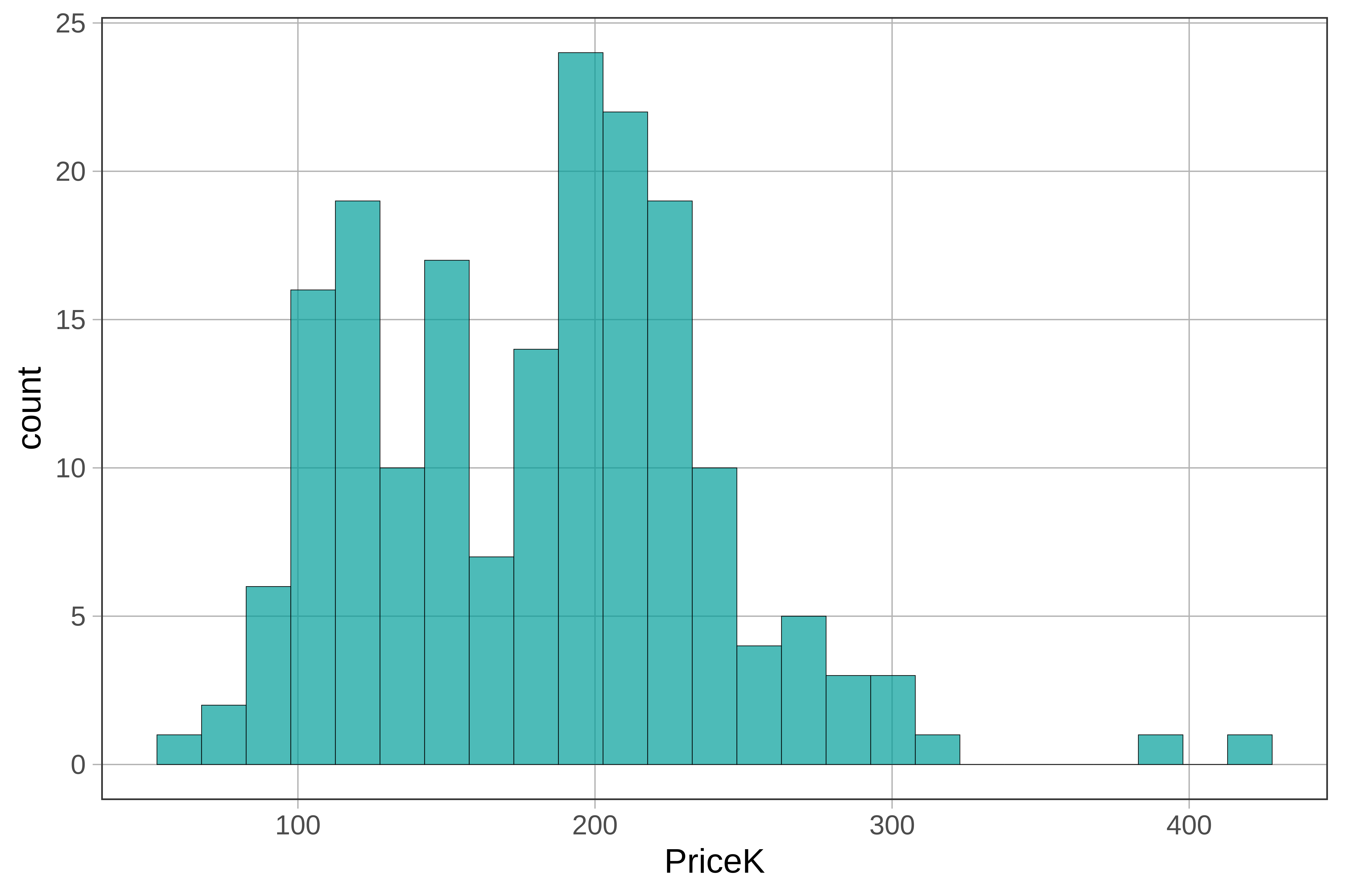
We can see from the histogram that sale prices of homes vary from under $100K to over $400K. What other variables might explain some of this variation we see in the sale price of homes?
One way to think about explaining variation in an outcome variable (like PriceK) is like this: if we knew a home’s value on some other variable (called the explanatory variable), that would help us make a better guess about the home’s value on the outcome variable (i.e., sale price).
Many of these variables might help us make better predictions about the home price! We’ll discuss a few of them in detail below.