2.7 DATA = MODEL + ERROR: Notation

Up to now we have represented models using word equations and R code. Now let’s go one step further to see how we can use mathematical notation to represent the simple (empty) model.

R code computes a model fit (e.g., \(b_0 = 181.4\)). Mathematical notation will help us represent the model that uses this value. This will be important as we move to more complex models.

We have introduced the overarching concept that DATA = MODEL + ERROR. In our simple model, we are using a simple mathematical function, the mean, to model the distribution of home prices. The function generates a single predicted price for every home in the distribution.

We could represent this model in a word equation like this:

PriceK = Mean + Error

Although math notation sometimes feels like it’s just here to make your life harder, there are some real advantages to rewriting this statement in mathematical notation. Here’s one form this notation might take:

\[Y_{i}=b_0+e_{i}\]

This equation comes from a statistical tradition called the General Linear Model (GLM). GLM equations are published in scientific articles (common in economics, biology, public health, etc.). We will use GLM notation throughout this book to help us represent and think about statistical models.

For the empty model of PriceK, the \(Y_i\) (pronounced “Y sub i”) represents the sale price for each home in the data set. \(Y_1\) is the price of the first home in the data set, \(Y_2\), the second home, and so on, up to \(Y_i\) for the last home in the data set. The \(b_0\) (“b sub 0”) represents the empty model prediction, and \(e_i\) is the error in prediction for each home in the data set.

For now, with the empty model, \(b_0\) represents the mean of PriceK (181.4). But for other models, and other situations, it can represent other values. Indeed, this flexibility is what makes the General Linear Model general. This will come in handy later when we make more complicated models.

Does DATA Really Equal MODEL + ERROR?

The GLM notation (\(Y_i = b_0 + e_i\)) literally represents that each value of \(Y\) in our data (\(Y_{i}\)) can be seen as the sum of two parts: the model’s predicted price (\(181.4K) and the residual from the prediction (\)e_{i}$, or error). If we add these two numbers together for a specific home price, we will get the original home price.

Let’s take a look at a single home in Ames that sold for $260K. In the plot below we have colored the dot representing this home black.

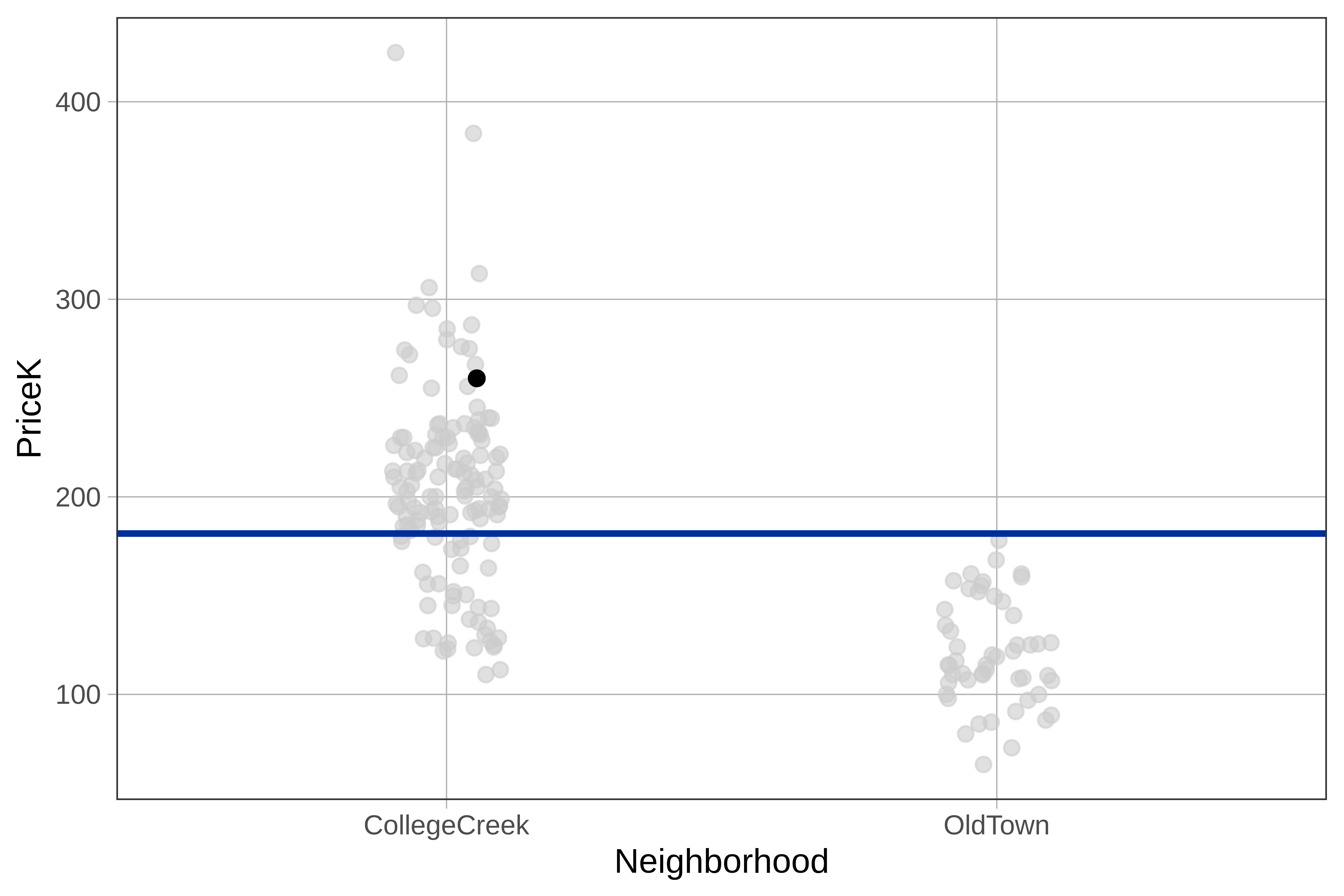
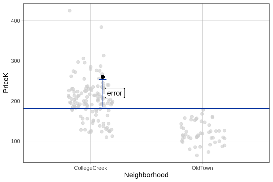
Using our simple model, we can decompose the price of the house we colored black into two parts, model and error. 260, therefore, can be expressed as 181.4 (the model prediction) + error. Put another way:

\[260 = 181.4 + e_i\]

Subtracting the data point from the model prediction will give us the error or residual (260 - 181.4 = 78.6). In this case, the residual is positive because this particular home’s price is higher than the price predicted by the empty model.

As our models become more complex they still will generate a predicted value of \(Y\) for each house. But whereas the empty model uses just the mean (thus predicting the same value for all the houses), more complex models will take other information into account (for example what neighborhood the house is in). The neighborhood model, for example, which we will develop in the next chapter, will predict a higher value for houses in one neighborhood and a lower one for houses in another neighborhood.