3.8 Interpreting the Parameter Estimates for a Regression Model
Previously, we used the lm() function to fit the HomeSizeK model of PriceK and saved it as HomeSizeK_model:
HomeSizeK_model` <- lm(PriceK ~ HomeSizeK, data = Ames)We used this model to generate predictions, but now let’s look at the parameter estimates and see how to interpret them.
We’ve already saved the model as HomeSizeK_model. Print its contents out in the code block below.
library(coursekata)
# saves the home size model
HomeSizeK_model <- lm(PriceK ~ HomeSizeK, data = Ames)

# print it out
# saves the home size model
HomeSizeK_model <- lm(PriceK ~ HomeSizeK, data = Ames)

# print it out
HomeSizeK_model
# temporary SCT
ex() %>% check_output_expr("HomeSizeK_model")Call:
lm(formula = PriceK ~ HomeSizeK, data = Ames)
Coefficients:
(Intercept) HomeSizeK
24.68 106.60 The Intercept corresponds to \(b_{0}\) and the HomeSizeK coefficient corresponds to \(b_{1}\). We can write our fitted model as:
\[PriceK_{i}=24.68 + 106.60HomeSizeK_{i}+e_{i}\]
Or, equivalently, using GLM notation, it can be written:
\[Y_{i}=24.68 + 106.60X_{i}+e_{i}\]
\(b_0\), which equals 24.68, is the y-intercept. It’s the predicted \(Y_i\) (PriceK) when \(X_i\) (HomeSizeK) equals 0.
How Regression Models Make Predictions
Similar to our use of the Neighborhood model, we can use the HomeSizeK model to predict the price at which a new home will sell. This time, however, we will adjust the prediction based on home size instead of neighborhood.
Recall that price (and predicted price) are in $1000 dollar units. The \(b_0\) (24.68 or $24,680) represents the predicted price for a home with a size of 0. If we stretch out the x-axis to include 0, we would expect the regression line to cross the y-axis at 24.68. (Notice, however, that in the plot below that there are no actual homes of size 0, for obvious reasons!)

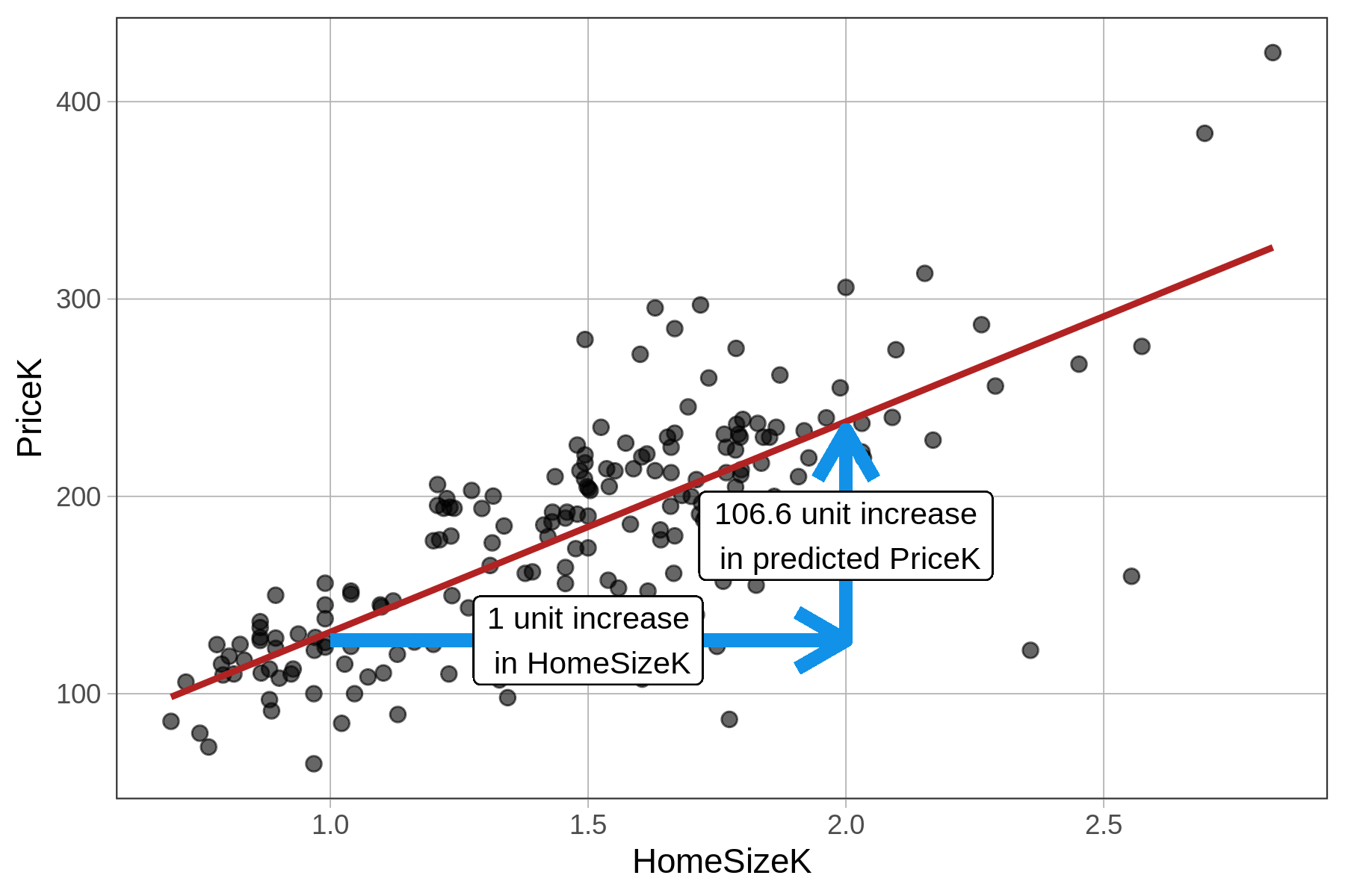
The \(b_1\) estimate (106.60) is the slope: for every 1 unit increase in HomeSizeK, our model predicts a 106.60 increase in PriceK. Because both of our variables represent units in thousands (HomeSizeK is thousands of square feet and PriceK is thousands of dollars), this means that homes with 1K more square feet are predicted by our model to have a $106.60K higher price tag (on average). Here’s a visual representation:
The predicted price of a 2.41K square foot home (that is, 2,410 square feet) is $281.59K. This is the \(Y_i\) (PriceK) on the regression line when \(X_i\) (HomeSizeK) is 2.41, as visualized below:

Comparing the Neighborhood Model and the HomeSizeK Model
Having now specified and fit two models, one a group model and the other a regression model, let’s just think for a bit on what the similarities and differences are between these models.
| Symbol |
Group Mean Model \({Price}_{i}=b_{0}+b_{1}{Neighborhood}_{i}+e_{i}\) |
Regression Model \({Price}_{i}=b_{0}+b_{1}{HomeSize}_{i}+e_{i}\) |
|---|---|---|
| \(Y_i\) | Price of home i | Price of home i |
| \(b_0\) |
Predicted home price when \(Neighborhood_i = 0\)) (mean home price in College Creek) |
Predicted home price when \(HomeSize_i=0\) (y-intercept for regression line) |
| \(b_1\) |
Adjustment to predicted price for a home in Old Town (the mean difference between the two group means) |
Adjustment to predicted price for a one-unit increase in home size (the slope of the regression line) |
| \(X_i\) | Neighborhood of home i, coded as 0=not-Old Town, 1=Old Town | Home size of home i in thousands of square feet |
| \(e_i\) | Error for home i | Error for home i |