5.7 Thinking About Error
We have developed the idea of the mean being the simplest (or empty) model of the distribution of a quantitative variable, represented in this word equation:
DATA = MEAN + ERROR
If this is true, then we can calculate error in our data set by just moving components of this equation around to get the formula:
ERROR = DATA - MEAN
Using this formula, if someone has a thumb length larger than the mean (e.g., 62 versus a mean of 60.1), then their error is a positive number (in this case, nearly +2). If they have a thumb length lower than the mean (e.g., 58) then we can calculate their error as a negative number (e.g. about -2).
We generally call the error calculated this way as the residual. Now that you know how to generate predictions, we’ll refine our definition of the residual to be the difference between our model’s prediction and an actual observed score. The word residual should evoke the stuff that remains because the residual is the leftover variation from our data once we take out the model.
To find these errors (or residuals) you can just subtract the mean from each data point. In R we could just run this code to get the residuals:
Fingers$Thumb - Fingers$PredictIf we run the code, R will calculate the 157 residuals, but it won’t save them unless we tell it to do so. Modify the code in the window below to save the residuals in a new variable in Fingers called Resid. (Note that the variable Predict already exists in the Fingers data frame).
require(coursekata)

Fingers$TinySet <- c(1,1,1,0,0,0,1,0,0,1, rep(0,147))
Fingers$TinySet[142] <- 1
Fingers <- arrange(arrange(Fingers, Height), desc(TinySet))

empty_model <- lm(Thumb ~ NULL, data = Fingers)
Fingers <- Fingers %>% mutate(
    Predict = predict(empty_model),
    Resid = Thumb - Predict
)
# modify this to save the residuals from the empty_model
Fingers$Resid <-

# this prints selected variables from Fingers
select(Fingers, Thumb, Predict, Resid)
Fingers$Resid <- Fingers$Thumb - Fingers$Predict
ex() %>% check_object("Fingers") %>%
check_column("Resid") %>% check_equal() Thumb Predict Resid
1 52 60.10366 -8.103662
2 56 60.10366 -4.103662
3 64 60.10366 3.896338
4 70 60.10366 9.896338
5 66 60.10366 5.896338
6 62 60.10366 1.896338These residuals (or “leftovers”) are so important in modeling that there is an even easier way to get them in R. The function resid(), when given a model (e.g., empty_model) will return all the residuals from the predictions of the model.
resid(empty_model)Modify the following code to save the residuals that we get using the resid() function as a variable in the Fingers data frame. Call the new variable EasyResid.
require(coursekata)

Fingers$TinySet <- c(1,1,1,0,0,0,1,0,0,1, rep(0,147))
Fingers$TinySet[142] <- 1
Fingers <- arrange(arrange(Fingers, Height), desc(TinySet))

empty_model <- lm(Thumb ~ NULL, data = Fingers)
Fingers <- Fingers %>% mutate(
    Predict = predict(empty_model),
    Resid = Thumb - Predict
)
# calculate the residuals from empty_model the easy way
# and save them in the Fingers data frame
Fingers$EasyResid <-

# this prints select variables from Fingers
head(select(Fingers, Thumb, Predict, Resid, EasyResid))
Fingers$EasyResid <- resid(empty_model)
Fingers
ex() %>% check_object("Fingers") %>%
check_column("EasyResid") %>% check_equal() Thumb Predict Resid EasyResid
1 52 60.10366 -8.103662 -8.103662
2 56 60.10366 -4.103662 -4.103662
3 64 60.10366 3.896338 3.896338
4 70 60.10366 9.896338 9.896338
5 66 60.10366 5.896338 5.896338
6 62 60.10366 1.896338 1.896338Notice that the values for Resid and EasyResid are the same for each row in the data set. We will generally use the resid() function from now on, just because it’s easier, but we want you to know what the resid() function is doing behind the scenes.
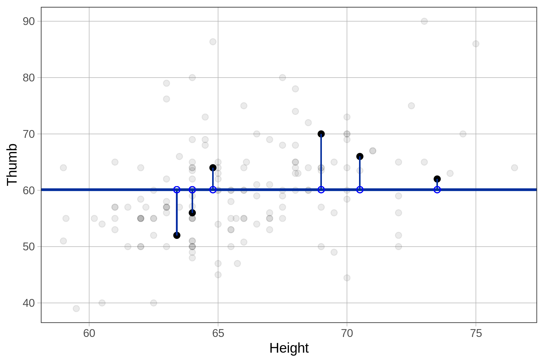
Below we have plotted a few of the residuals from the Fingers data set on the Thumb by Height scatterplot. Visually, the residuals can be thought of as the vertical distance between the data (the students’ actual thumb lengths) and the model’s predicted thumb length (60.1).
Note that sometimes the residuals are negative (extending below the empty model) and sometimes positive (above the empty model). Because the empty model is the mean, we know that these residuals are perfectly balanced across the full data set of 157 students.
Distribution of Residuals
Below we’ve plotted histograms of the three variables: Thumb, Predict, and Resid.
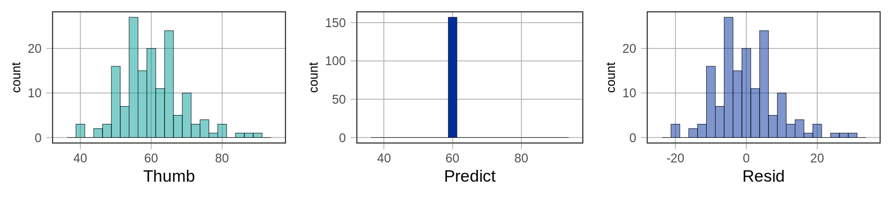
The distributions of the data and the residuals have the same shape. But the numbers on the x-axis differ across the two distributions. The distribution of Thumb is centered at the mean (60.1), whereas the distribution of Resid is centered at 0. Data that are smaller than the mean (such as a thumb length of 50) have negative residuals (-10) but data that are larger than the mean (such as 70) have positive residuals (10).
Let’s see what we would get if we summed all values for the variable Fingers$Resid. Try it in the code block below.
require(coursekata)

empty_model <- lm(Thumb ~ NULL, data = Fingers)
Fingers <- Fingers %>% mutate(
    Predict = predict(empty_model),
    Resid = resid(empty_model)
)
# assume Fingers data frame already has the variable Resid saved in it
sum(Fingers$Resid)
ex() %>% {

    check_output_expr(., "sum(Fingers$Resid)")
}-1.4738210651899e-14R will sometimes give you outputs in scientific notation. The -1.47e-14 is equivalent to \(-1.47*10^{-14}\) which indicates that this is a number very close to zero (the -14 meaning that the decimal point is shifted to the left 14 places)! Whenever you see this scientific notation with a large negative exponent after the “e”, you can just read it as “zero,” or pretty close to zero.
The residuals (or error) around the mean always sum to 0. The mean of the errors will also always be 0, because 0 divided by n equals 0. (R will not always report the sum as exactly 0 because of computer hardware limitations but it will be close enough to 0.)