9.3 Interpreting the Parameter Estimates for a Regression Model
Previously, we used the lm() function to fit the Height model of Thumb and saved it as Height_model:
Height_model <- lm(Thumb ~ Height, data = Fingers)Let’s now look at the parameter estimates for this model and see how to interpret them. Use the code block below to print out the parameter estimates for the height model.
library(coursekata)
# saves the Height model
Height_model <- lm(Thumb ~ Height, data = Fingers)

# print it out
# saves the Height model
Height_model <- lm(Thumb ~ Height, data = Fingers)

# print it out
Height_model
ex() %>% check_output_expr("Height_model")Call:
lm(formula = Thumb ~ Height, data = Fingers)
Coefficients: (Intercept) Height

-3.3295 0.9619The Intercept corresponds to \(b_0\) and the Height coefficient corresponds to \(b_1\). We can write our fitted model as:
\[\text{Thumb}_i=-3.33 + 0.96\text{Height}_i+e_i\]
Or, equivalently, using GLM notation, it can be written:
\[Y_i=-3.33 + 0.96X_i+e_i\]
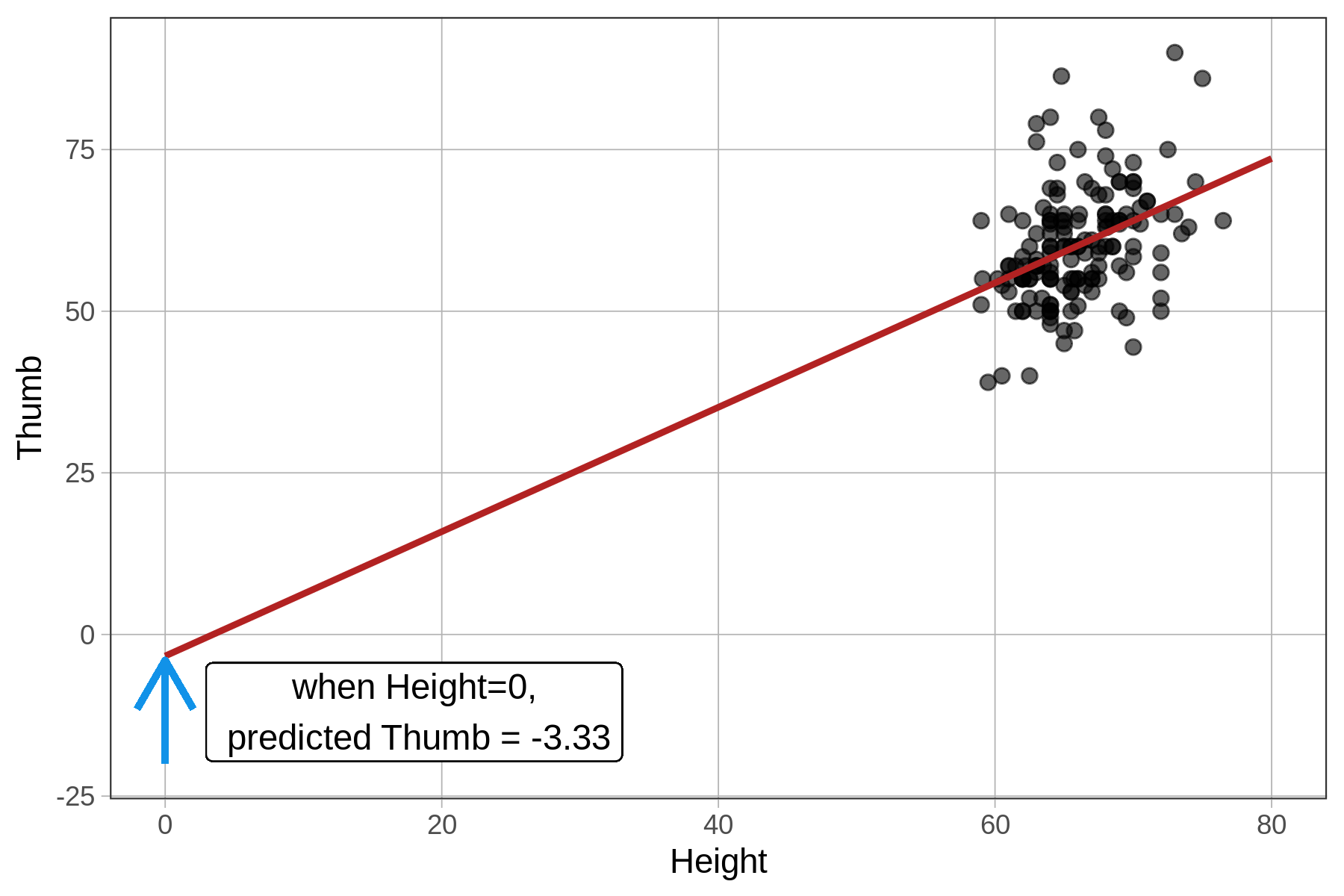
\(b_0\), which is -3.33, is the y-intercept. It’s the predicted \(Y_i\) (Thumb) when \(X_i\) (Height) equals 0.
Neither a height of 0 inches nor a thumb length of -3.33 mm are possible. Not all predictions from a regression model make sense. We should always be thinking about which values of the predictors, and which predictions, are reasonable.
How Regression Models Make Predictions
We can use the Height model to predict the thumb length of students of different heights (just like we used the Height2Group model to predict the thumb length of short and tall groups of students).
Recall that thumb length (and predicted thumb length) are expressed in millimeters. \(b_0\) (-3.33) is the predicted thumb length in millimeters for a student with a height of 0 inches. If we stretch out the x-axis to include 0, we would expect the regression line to cross the y-axis at -3.33. (Notice, however, that in the plot below that there are no actual students who are 0 inches in height, for obvious reasons!)
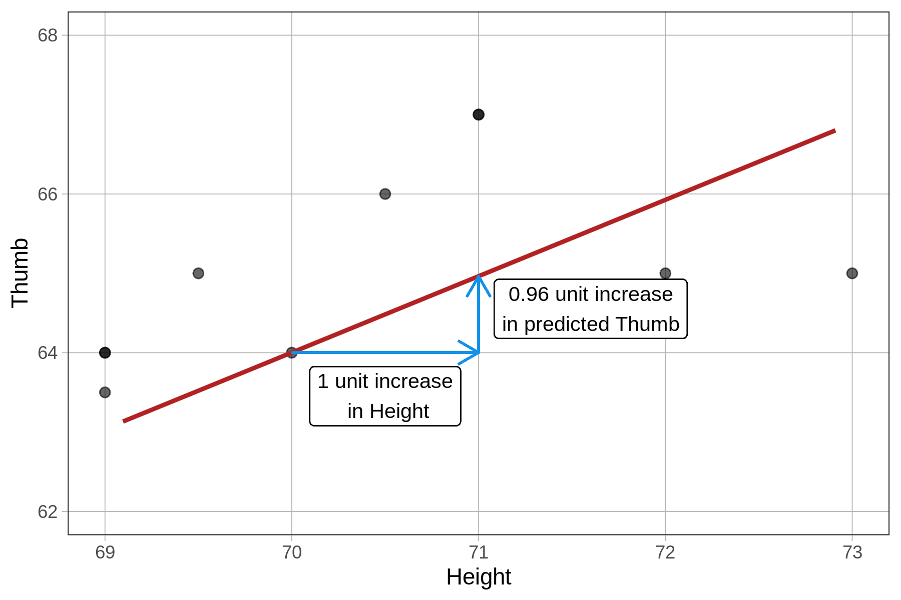
The \(b_1\) estimate (0.96) is the slope: for every 1 unit increase in Height, our model predicts a 0.96 unit increase in Thumb. The fact that height is measured in inches and thumb length in millimeters is not a problem; the regression line is a function (the \(b_0 + b_1Height_i\) part) that takes in inches and then makes a prediction in millimeters. This means that students who are 1 inch taller are predicted by our model to have thumbs that are 0.96 millimeters longer (on average). Here’s a visual representation:
| default scale | zooming in |
|---|---|
|
|
|

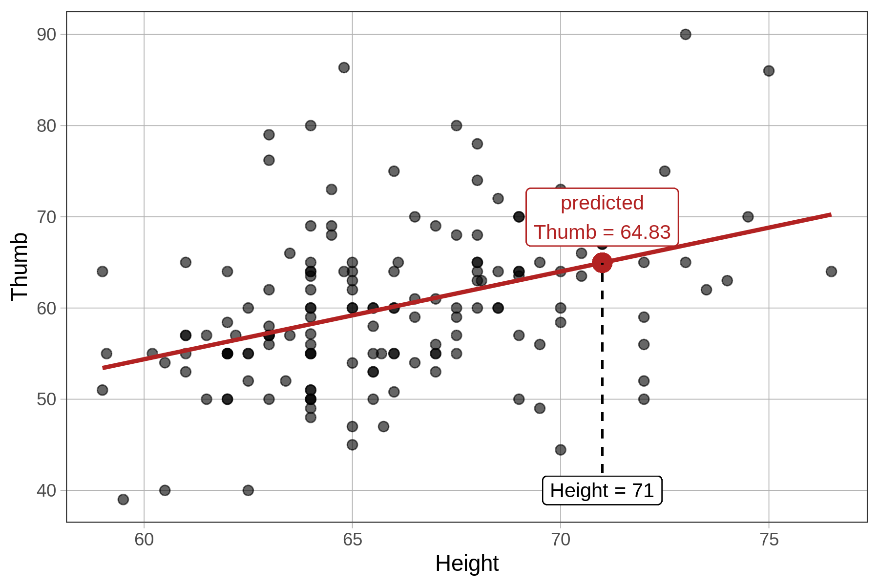
The predicted thumb length of a student who is 71 inches tall is 64.83 mm. This is the value of \(Y\) (Thumb) on the regression line when \(X\) (Height) is 71, as visualized below:
Regression Coefficients are Not Symmetrical
When you fit a regression model, it matters which variable is the outcome and which is the explanatory variable. For example, if you fit the model Thumb ~ Height you won’t get the same y-intercept and slope you would if you fit the model Height ~ Thumb.
|
Coefficients: (Intercept) Height
|
Coefficients: (Intercept) Thumb
|
The reason for this is that the units, and the distributions of the variables, are different. If the outcome is Thumb, then the slope is the adjustment to predicted thumb length for a one-inch increase in height. But if the outcome is height, then the slope is the adjustment to predicted height length for a one-millimeter increase in thumb length. These are two entirely different things.