9.9 More on Pearson’s r
Producing a Correlation Matrix
One nice thing about correlations is that they can summarize the strengths of linear relationships across many pairs of variables. We’ve learned how to calculate a single correlation coefficient; let’s now learn how to create a matrix of correlations.
Using select(), we’ve created a new data frame called Hand with just a few of the variables from the Fingers data frame.
Hand <- select(Fingers, Thumb, Index, Middle, Ring, Pinkie, Height)
head(Hand)
Thumb Index Middle Ring Pinkie Height
1 66.00 79.0 84.0 74.0 57.0 70.5
2 64.00 73.0 80.0 75.0 62.0 64.8
3 56.00 69.0 76.0 71.0 54.0 64.0
4 58.42 76.2 91.4 76.2 63.5 70.0
5 74.00 79.0 83.0 76.0 64.0 68.0
6 60.00 64.0 70.0 65.0 58.0 68.0In the code window below, enter the cor() command as before, but this time instead of putting in the specific variables, just put in the name of a data frame (in this case, use Hand). Run it and see what happens.
require(coursekata)

Fingers <- Fingers %>%
    filter(Thumb >= 33 & Thumb <= 100) %>%
    mutate(
        zThumb = zscore(Thumb),
        zHeight = zscore(Height)
    )

Hand <- select(Fingers, Thumb, Index, Middle, Ring, Pinkie, Height)
# run the cor() function with the Hand data frame
cor(Hand)
ex() %>% check_function("cor") %>% check_result() %>% check_equal() Thumb Index Middle Ring Pinkie Height
Thumb 1.0000000 0.7788568 0.7479010 0.6999031 0.6755136 0.3910649
Index 0.7788568 1.0000000 0.9412202 0.8820600 0.7825979 0.4974643
Middle 0.7479010 0.9412202 1.0000000 0.8945526 0.7475880 0.4737641
Ring 0.6999031 0.8820600 0.8945526 1.0000000 0.8292530 0.4953183
Pinkie 0.6755136 0.7825979 0.7475880 0.8292530 1.0000000 0.5695369
Height 0.3910649 0.4974643 0.4737641 0.4953183 0.5695369 1.0000000This returns a whole matrix, each number representing a correlation coefficient (\(r\)) for the pair of variables. We have highlighted a familiar one (\(r=0.39\)) the correlation between thumb length and height which is printed in two places in the matrix).
Correlations, because they are based on standardized variables, are symmetrical in that the correlation of Thumb and Height is the same as the correlation between Height and Thumb.
Notice that each variable is perfectly correlated (\(r=1.0\)) with itself. If you look diagonally down the correlation matrix, you’ll see a bunch of 1’s.
\(R^2\) and PRE
You may recall that we told you that PRE goes by another name in some quarters: \(R^2\). Here’s a fun fact: if you fit a regression model, print out the supernova() table, and then take the square root of the PRE, you will get Pearson’s \(r\).
Go ahead and give it a try. Here is the supernova table for the height model of Thumb. Note that the PRE is .1529.
Analysis of Variance Table (Type III SS)
Model: Thumb ~ Height

                               SS  df       MS      F    PRE     p
----- --------------- | --------- --- -------- ------ ------ -----
Model (error reduced) |  1816.862   1 1816.862 27.984 0.1529 .0000
Error (from model)    | 10063.349 155   64.925
----- --------------- | --------- --- -------- ------ ------ -----
Total (empty model)   | 11880.211 156   76.155
Use the code window below to take the square root of .1529, and then use the cor() function to calculate Pearson’s r for the two variables. Do the two results match? They should!
require(coursekata)

Fingers <- Fingers %>%
    filter(Thumb >= 33 & Thumb <= 100) %>%
    mutate(
        zThumb = zscore(Thumb),
        zHeight = zscore(Height)
    )
# this code finds the square root of the PRE.1529
sqrt(.1529)

# add code to calculate the correlation between Thumb and Height
# this code finds the square root of .1529
sqrt(.1529)
# add code to calculate the correlation between Thumb and Height
cor(Thumb ~ Height, data = Fingers)
ex() %>% check_output_expr("cor(Thumb ~ Height, data = Fingers)")0.391064927516154
0.391064927516154Regression analyses will often report \(R^2\). \(R^2\) is just another name for PRE when the complex model is being compared to the empty model. (\(R^2\) won’t help you if in the future you want to compare one complex model to another complex model.)
Like PRE, Pearson’s \(r\) is just a sample statistic; it is only an estimate of the true correlation in the population.
Comparing the Fit of Standardized and Unstandardized Regression Models
You’ve learned a lot about the correlation coefficient which comes from the standardized regression model. You might wonder – is it that this is a “better” regression model, as in, does it explain more variation than the unstandardized one?
Unstandardized: Thumb ~ Height
|
Standardized: zThumb ~ zHeight
|
|---|---|
|
|
|
We have printed the two ANOVA tables below. Compare them carefully to see what is the same, and what is different, between the two models.
Unstandardized Model
Analysis of Variance Table (Type III SS)
Model: Thumb ~ Height

                               SS  df       MS      F    PRE     p
----- --------------- | --------- --- -------- ------ ------ -----
Model (error reduced) |  1816.862   1 1816.862 27.984 0.1529 .0000
Error (from model)    | 10063.349 155   64.925
----- --------------- | --------- --- -------- ------ ------ -----
Total (empty model)   | 11880.211 156   76.155
Standardized Model
Analysis of Variance Table (Type III SS)
Model: zThumb ~ zHeight
SS df MS F PRE p
----- --------------- | ------- --- ------ ------ ------ -----
Model (error reduced) | 23.857 1 23.857 27.984 0.1529 .0000
Error (from model) | 132.143 155 0.853
----- --------------- | ------- --- ------ ------ ------ -----
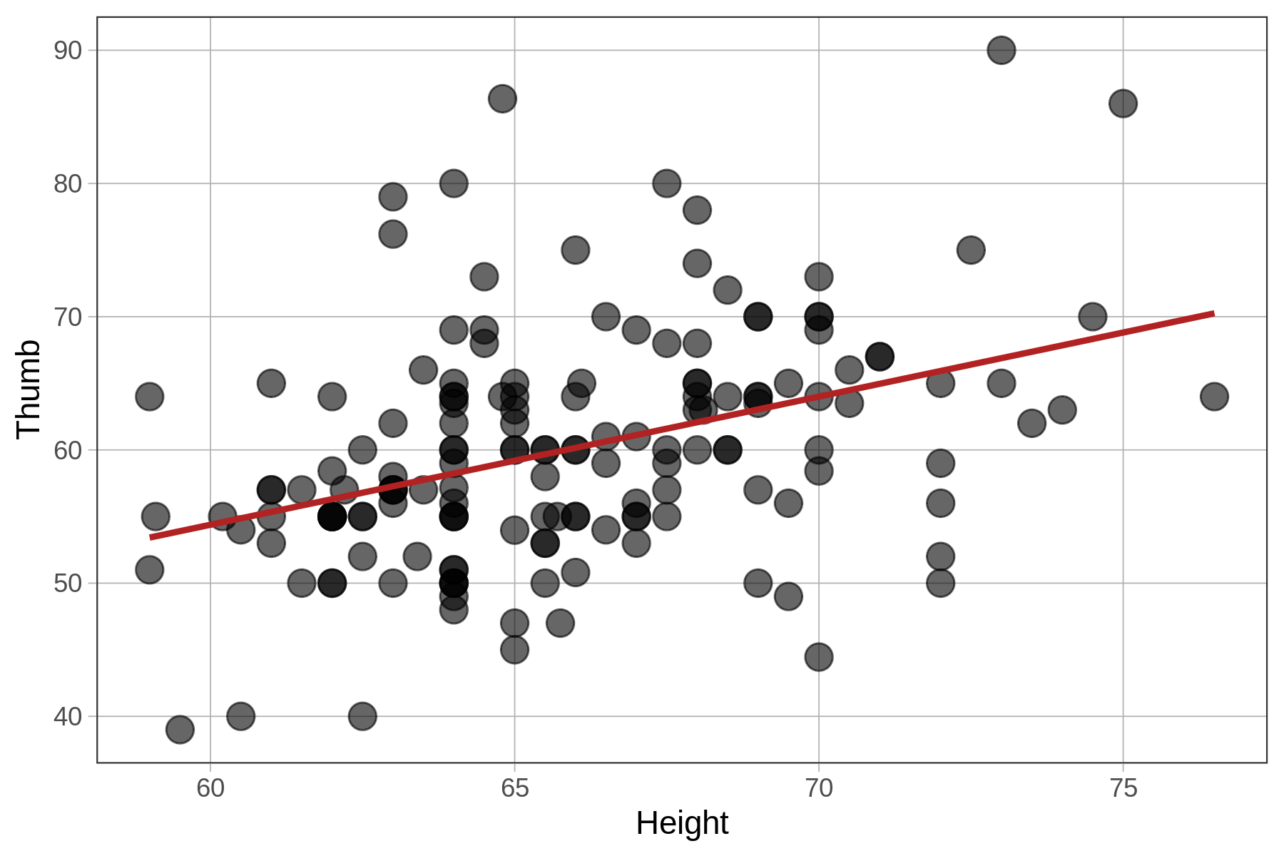
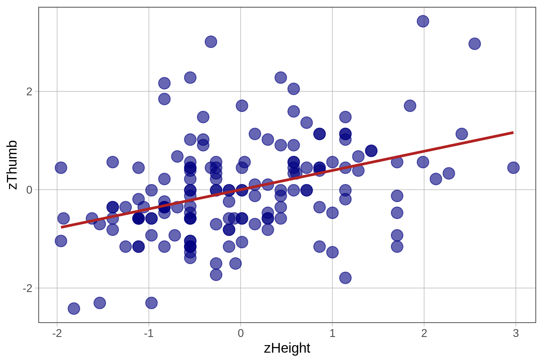
Total (empty model) | 156.000 156 1.000 The fit of the models (measured with PRE and F) is identical because all we have changed is the unit in which we measure the outcome and explanatory variables. The z-transformation does not change the shape of the bivariate distribution, as represented in the scatterplot, at all. It simply changes the scale on both axes to standard deviations instead of inches and millimeters.
Unlike PRE and F, which are proportions and ratios, respectively, SS are expressed in the units of the measurement. So if we converted the mm (for Thumb length) and inches (for Height) into cm, feet, standard deviations, etc, the SS would change to reflect those new units.