Chapter 9 - Models with a Quantitative Explanatory Variable

9.1 Using a Quantitative Explanatory Variable in a Model

Height2Group is a categorical variable. The Height2Group model is what we might call a group model because it uses the group mean as the best prediction of thumb lengths for each group (in this case, short and tall people).

Not all models are group models, however. If we want to use a quantitative variable as an explanatory variable we will need to adjust our model a bit. Models that use quantitative predictors are often referred to as regression models.

The Height Model of Thumb

One quantitative variable in the Fingers data frame that might explain some of the variation in Thumb is Height: the height of a student in inches. (Note: Height is measured in inches but Thumb is measured in millimeters.)

Previously, we created a scatterplot to visualize the relationship between Thumb and Height. We’ve reprinted that scatterplot below.

gf_point(Thumb ~ Height, data = Fingers)

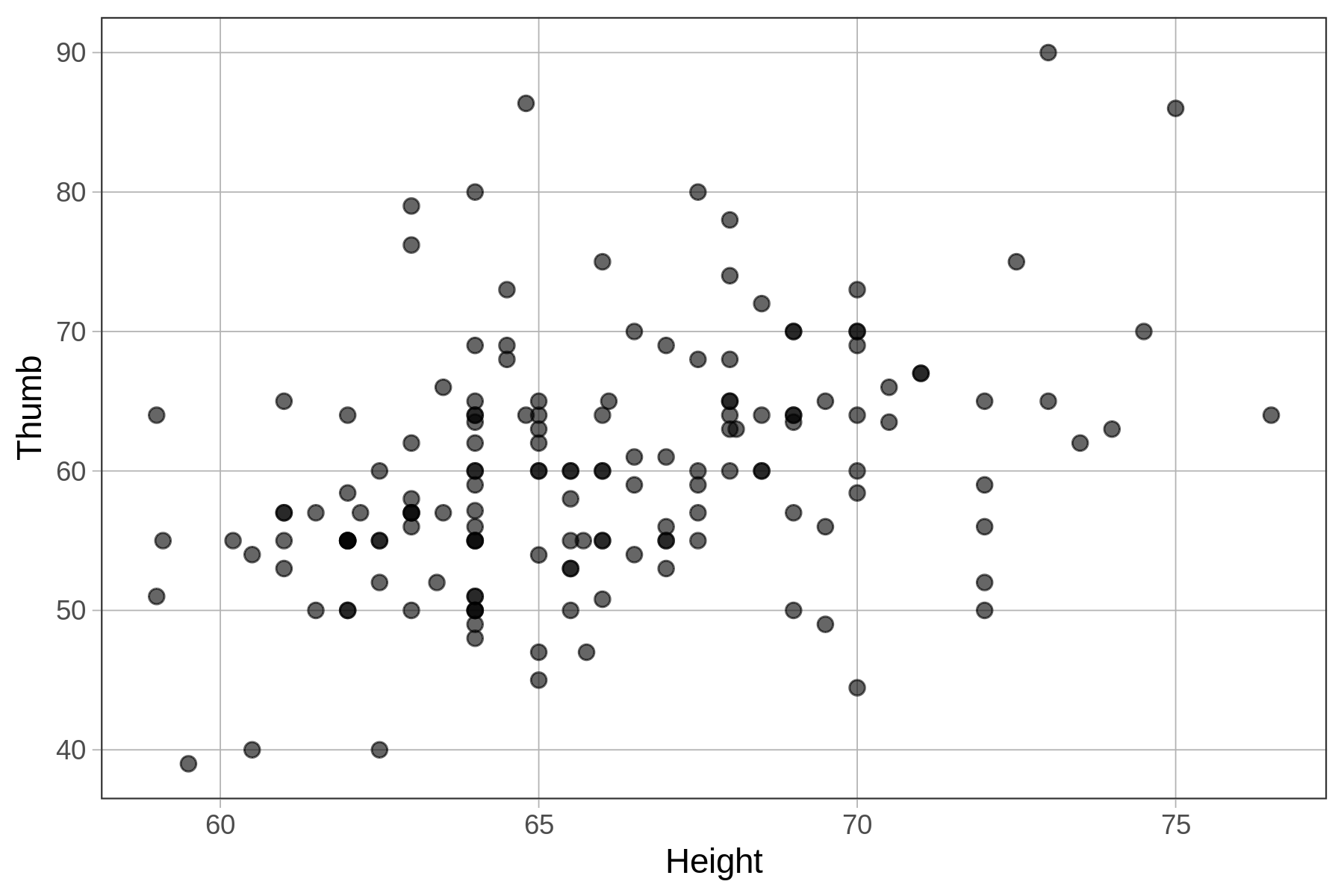
As we noted previously, it does appear that if we know the height of a student we can make a better guess as to their thumb length than if we didn’t have this information. Taller students tend to have longer thumbs, and shorter students, shorter thumbs. We call a pattern like this a positive relationship because as one variable goes up, so does the other.

If we want to make specific predictions, and quantitatively compare the Height model to other models, we need to turn it into a statistical model, much like we did when we developed the Height2Group model. This time, however, we can’t use group means as the model predictions because there are no groups! Instead, we will use a line, called the regression line, to make predictions.

A regression line is the simplest way to model the relationship between two quantitative variables. We overlaid the best-fitting regression line (or model) on the scatterplot below. This line shows the predicted thumb length of a student based on their height.

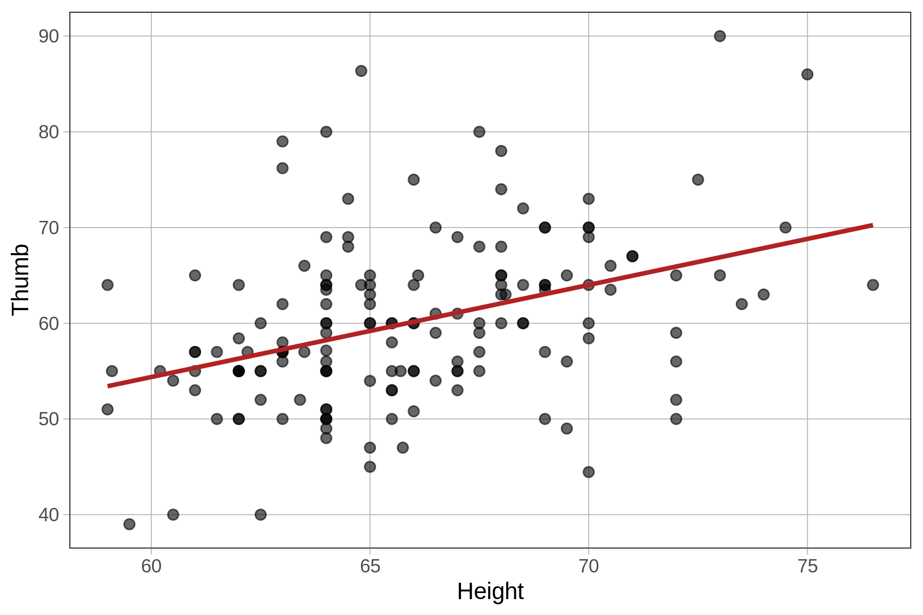
We will learn how to fit a regression model (i.e., find the best-fitting line) using R in a moment, but first it’s worth pointing out that the regression line is not just any line, just like the mean is not just any number.

Just as the group means are the points at which the sum of squared residuals are minimized for a group model, the regression line is the exact line, defined by its slope and y-intercept, from which the residuals are balanced and the sum of squared residuals is minimized for a model with a quantitative outcome and a quantitative predictor. Let’s dig into what that really means.

Predictions from the Height Model

We will use the lm() function to fit the Height model in the same way we did with the group model. You don’t have to tell R that this is a regression model; R will guess, just based on the fact that your explanatory variable is quantitative, not categorical.

Use the code window below to fit the Height model using lm(), and then save it into an object called Height_model. Then add some code to generate the model predictions, and save them as a new column in the Fingers data frame. (HINT: Consider using the predict() function.)

 Thumb Height Height_predict
1 66.00   70.5       64.48330
2 64.00   64.8       59.00056
3 56.00   64.0       58.23105
4 58.42   70.0       64.00235
5 74.00   68.0       62.07859
6 60.00   68.0       62.07859

We ran the code below to overlay the predicted thumb lengths of the Height model onto the original scatterplot depicting the actual thumb lengths. (The predictions are represented by red circles, accomplished by adding arguments for shape and color to the gf_point() function .)

Fingers$prediction <- predict(Height_model)
 
gf_point(Thumb ~ Height, data = Fingers) %>%
  gf_point(prediction ~ Height, shape = 1, size = 3, color = "firebrick")

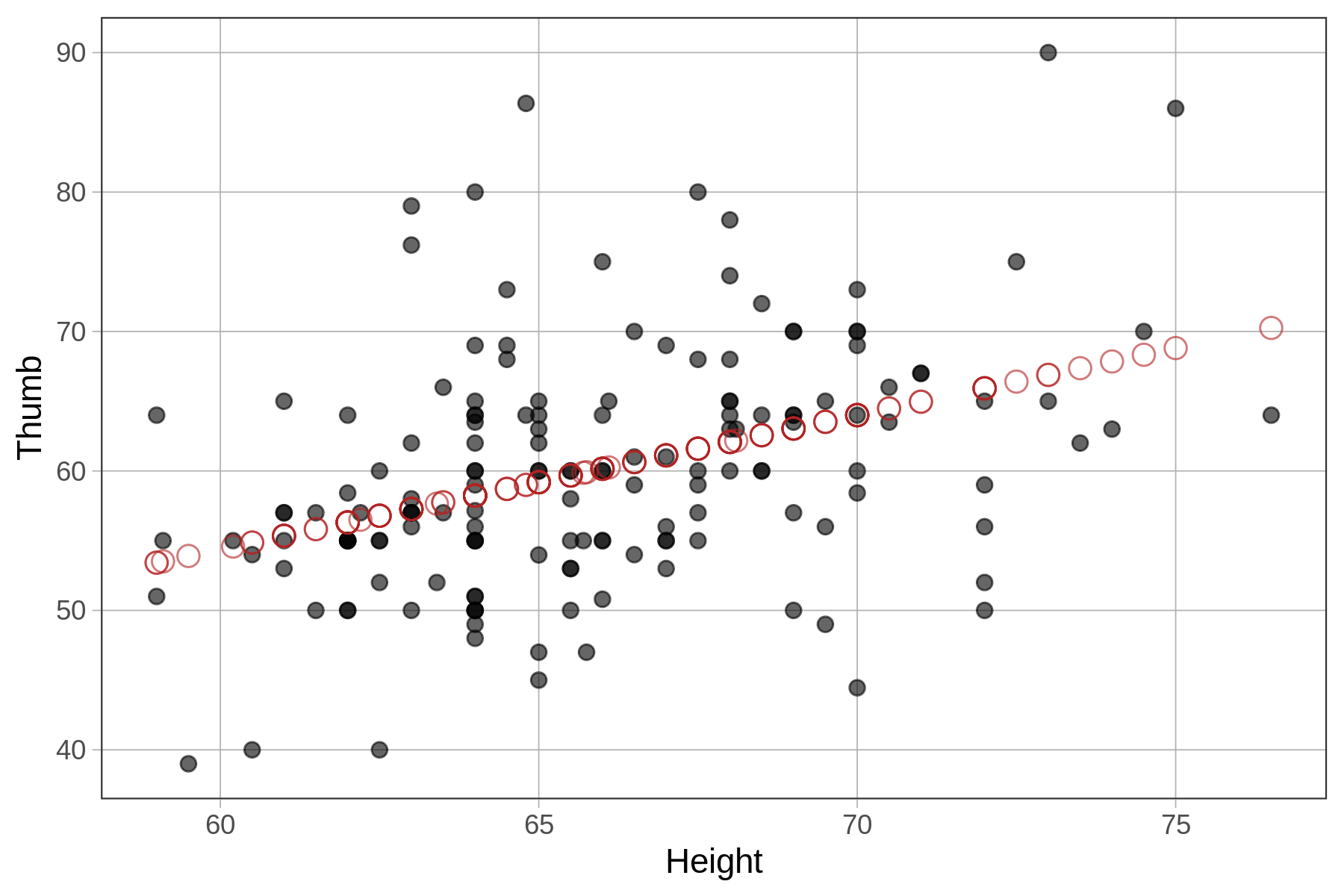
Each value of Height (e.g., 61, 62, 63) in the data set gets a unique model prediction (represented by the red circles). See how all the predictions seem to fall in a straight line? This is no accident! It’s because the predictions were generated by the regression line that R fit to the data.

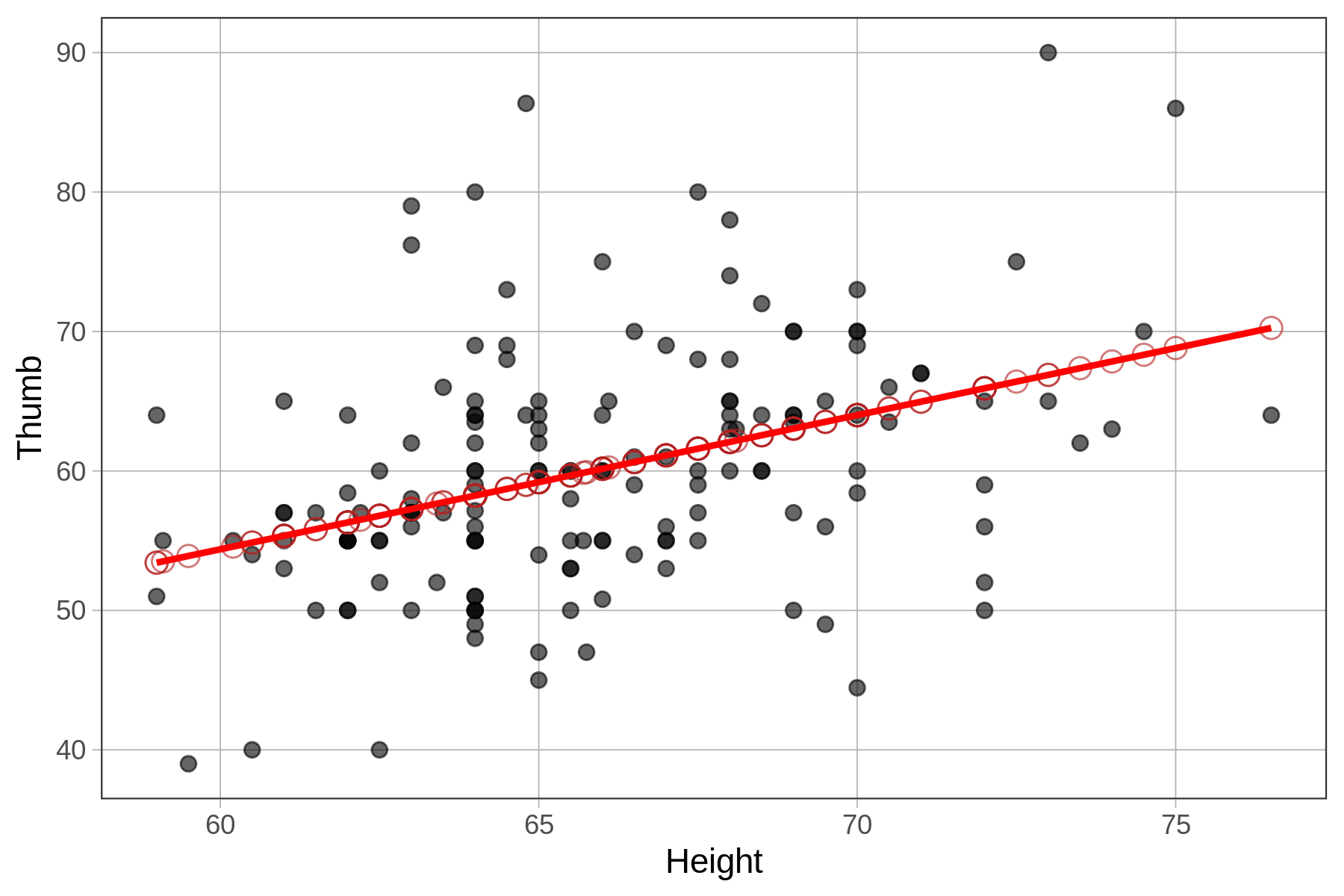
If we chain on gf_model() to our scatterplot, the best fitting model lies right on top of the model predictions.

gf_point(Thumb ~ Height, data = Fingers) %>%
  gf_point(prediction ~ Height, shape = 1, size = 3, color = "firebrick") %>%
  gf_model(Height_model, color="red")

Note that there are at least two ways to overlay a regression model onto a scatterplot. The first is by using gf_model(), which requires that we specify the model we want to see on the plot (e.g., gf_model(Height_model)). The advantage of gf_model() is that it works for group models as well as regression models.

Another way is to chain on the function gf_lm() to the scatterplot. This method doesn’t require you to specify a model (it figures that out from information in the scatterplot), but it only works for regression models.