7.8 Using SS Error to Compare the Group Model to the Empty Model
To calculate the sum of squares error for each model, we don’t have to add a new column to the data frame. We can, instead, just generate the residuals from each model, then square them and sum them.
In the code window below we have entered code to calculate the SS Total for the empty model. Add some code to calculate SS Error for the Sex model. (We already have created and saved the two models: empty_model and Sex_model.)
require(coursekata)
# This codes saves the best fitting models
empty_model <- lm(Thumb ~ NULL, data=Fingers)
Sex_model <- lm(Thumb ~ Sex, data=Fingers)

# This code squares and sums the residuals from the empty model
sum(resid(empty_model)^2)

# Write code to square and sum the residuals from the Sex model
# This codes saves the best fitting models
empty_model <- lm(Thumb ~ NULL, data=Fingers)
Sex_model <- lm(Thumb ~ Sex, data=Fingers)

# This code squares and sums the residuals from the empty model
sum(resid(empty_model)^2)

# Write code to square and sum the residuals from the Sex model
sum(resid(Sex_model)^2)
ex() %>% {
  check_function(., "sum", 1) %>%
    check_result() %>% check_equal()
  check_function(., "sum", 2) %>%
    check_result() %>% check_equal()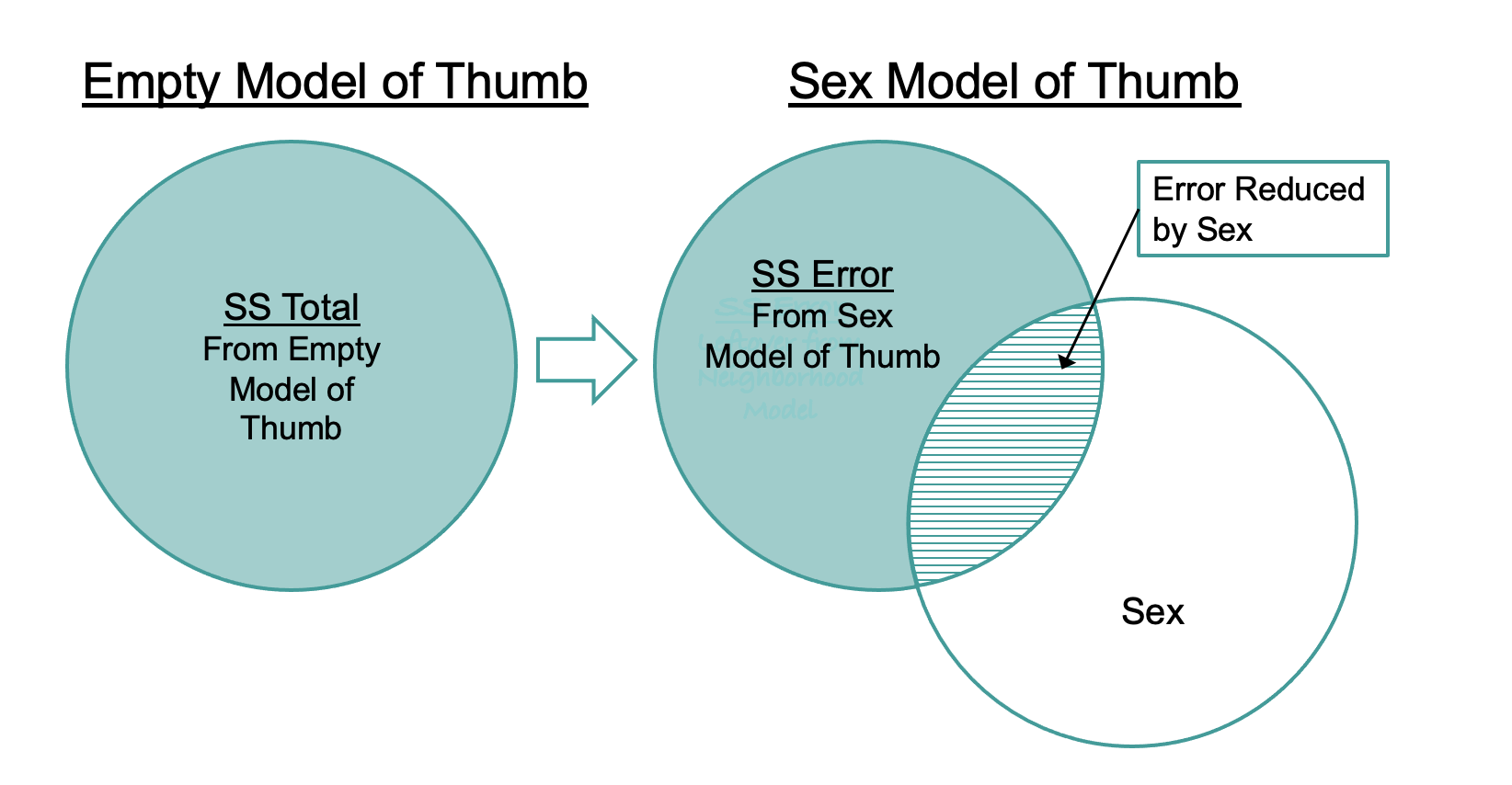
}11880.210919108310546.0083744196We can see from this output that we have, indeed, reduced our error by adding Sex as an explanatory variable into the model. Whereas the sum of squared errors around the empty model (SS Total) was 11,880, for the Sex model (SS Error) it was 10,546. We now have a quantitative basis on which to say that the Sex model is a better model of our data than the empty model.
This idea is visualized in the figure below.
Using supernova() to Calculate SS Error
Although we have been building these calculations from the residuals up, we now will show you an easier way to summarize the various sums of squares using ANOVA (ANalysis Of VAriance) tables.
We introduced the supernova() function earlier as a way of getting SS Total for the empty model. We can use the same function to calculate the SS Error (and more!) from the Sex model and other group models.
We have created and saved two models in the code window below: empty_model and Sex_model . Run the code as is and you will get the ANOVA table for the empty_model. Modify the supernova() code to get the ANOVA table for the Sex_model.
require(coursekata)
empty_model <- lm(Thumb ~ NULL, data = Fingers)
Sex_model <- lm(Thumb ~ Sex, data = Fingers)

# try running the code as is
# then modify to create the ANOVA table for Sex_model
supernova(empty_model)
empty_model <- lm(Thumb ~ NULL, data = Fingers)
Sex_model <- lm(Thumb ~ Sex, data = Fingers)
supernova(Sex_model)
ex() %>% {
    check_function(., "lm") %>% check_result() %>% check_equal()
    check_object(., "Sex_model") %>% check_equal()
    check_function(., "supernova") %>% check_result() %>%  check_equal()
}
Analysis of Variance Table (Type III SS)
 Model: Thumb ~ Sex

                                SS  df       MS      F    PRE     p
 ----- --------------- | --------- --- -------- ------ ------ -----
 Model (error reduced) |  1334.203   1 1334.203 19.609 0.1123 .0000
 Error (from model)    | 10546.008 155   68.039
 ----- --------------- | --------- --- -------- ------ ------ -----
 Total (empty model)   | 11880.211 156   76.155
Although there is a lot going on in this table, the highlighted numbers are the SS Error and SS Total that we previously calculated from the residuals. Notice that the ANOVA table for Sex_model calculates both the SS Error (labeled Error) and the SS Total (labeled Total, the error from the empty model).
SS Total is the smallest SS we could have without adding an explanatory variable to the model. It represents the total variation in the outcome variable that we would want to explain. Taking that as our starting point, we can reduce the error by adding an explanatory variable into the model (in this case Sex).
Adding an explanatory variable to the model can decrease the sum of squares for error, but it can’t increase it. If the new model does not make better predictions than the empty model then the sum of squares would stay the same. But it’s rare for an explanatory variable to have no predictive value at all.