6.5 Confidence Intervals for Other Parameters

We have spent a lot of time working with the confidence interval for \(b_1\) in the two-group model, the model that we used to explain variation in the tipping experiment. But we can create confidence intervals for other parameters as well.

We don’t typically create confidence intervals around F because the F-distribution is not symmetrical, making the confidence interval harder to interpret. But for any of the parameters we label with a \(\beta\) we can use the same methods to find the confidence interval. Let’s look at a few examples.

The Confidence Interval for \(\beta_0\)

In the tipping study, we have put most of our emphasis on the confidence interval for the effect of smiley face on Tip, represented as \(\beta_1\). But we also are estimating another parameter in this two-group model: \(\beta_0\). The complete model we are trying to estimate looks like this:

\[Y_i=\beta_0+\beta_{1}X_i+\epsilon_i\]

The \(\beta_0\) parameter is the mean Tip for the control group in the study. If we fit and then run confint() on this model, we get 95% confidence intervals for both the \(\beta_0\) and \(\beta_1\) parameters.

You’ve seen this output before when we used confint() to get the confidence interval for \(\beta_1\).

                         2.5 %   97.5 %
(Intercept)          22.254644 31.74536
ConditionSmiley Face -0.665492 12.75640

This time we will focus on the line labeled (Intercept), because that shows us the confidence interval for \(\beta_0\). (It’s called the intercept because it’s the predicted value of Tip when \(X_i=0\).)

\(\beta_0\) represents the average tip in the DGP for tables that do not get smiley faces. It’s the population mean for tables in the control group. The confidence interval around \(\beta_0\) acknowledges that although the best point estimate for the control group mean in the DGP is our \(b_0\), we are 95% confident that the true value is between $22.25 and $31.75.

What if you wanted to find the confidence interval for \(\beta_0\) for the empty model of Tip? In other words, what would be the average amount tipped by all tables (both control and smiley face) in the DGP? What is the confidence interval for this average tip? Again, we can use confint(), which can take in any type of model.

               2.5 %   97.5 %
(Intercept) 26.58087 33.46459

In the table below we show the confint() output for both the condition model and the empty model.

confint(Condition_model)

confint(empty_model)

                         2.5 %   97.5 %
(Intercept)          22.254644 31.74536
ConditionSmiley Face -0.665492 12.75640

               2.5 %   97.5 %
(Intercept) 26.58087 33.46459

The condition model had two parameters (\(\beta_0\) and \(\beta_1\)) whereas the empty model had only one (\(\beta_0\)). confint() will calculate the confidence intervals for each parameter in the model so it will return different lines of output depending on the number of parameters.

Notice that the confidence interval around \(\beta_0\) from the empty model goes from $26.58 to $33.46, meaning that we can be 95% confident that the true mean tip in the DGP is between these two boundaries.These numbers are different from the confidence interval around \(\beta_0\) from the Condition model ($22.25 and $31.75).

The Confidence Interval for the Slope of a Regression Line

Let’s go back to the regression model we fit using total Check to predict Tip. We can specify this model of the DGP like this:

\[Y_i=\beta_0+\beta_{1}X_i+\epsilon_i\]

Here is the output for the best-fitting Check model using lm().

Call:
lm(formula = Tip ~ Check, data = TipExperiment)

Coefficients:
(Intercept)        Check
   18.74805      0.05074

Use the code window below to find the confidence interval for the slope of this regression line.

                 2.5 %      97.5 %
(Intercept) 12.76280568 24.73328496
Check        0.02716385  0.07431286

The \(\beta_1\) represents the increment that is added to the predicted tip in the DGP for every additional dollar spent on the total check. The confidence interval of \(\beta_1\) represents the range of \(\beta_1\)s that would be likely to produce the sample \(b_1\). About 3 cents is the lowest \(\beta_1\) that would be likely to produce the sample \(b_1\) and 7 cents is the highest.

Now that we have tried confint(), try using the resample() function to bootstrap the 95% confidence interval for the slope of the regression line. See how your bootstrapped confidence interval compares to the results obtained by using confint().

Here is a histogram of the bootstrapped sampling distribution we created. Yours will be a little different, of course, because it is random.

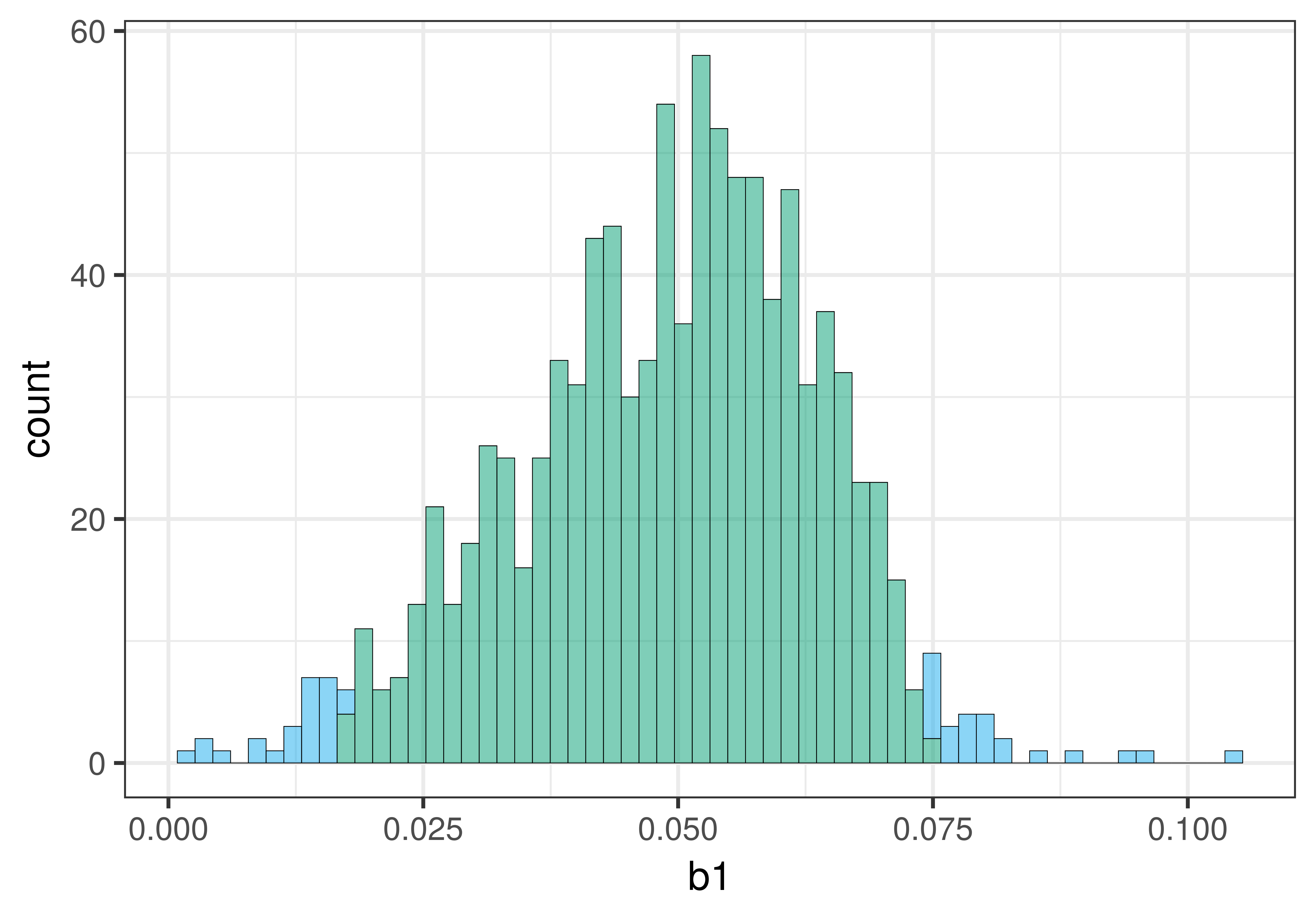
The center of the bootstrapped sampling distribution is approximately the same as the sample \(b_1\) of .05. This is what we would expect because bootstrapping assumes that the sample is representative of the DGP.

As explained previously, we can use the .025 cutoffs that separate the unlikely tails from the likely middle of the sampling distribution as a handy way to find the lower and upper bound of the 95% confidence interval. We can eyeball these cutoffs by looking at the histogram, or we can calculate them by arranging the bootstrapped sampling distribution to find the actual 26th and 975th b1s.

0.0172834762542693
0.0757609233182571

To find the confidence interval, we sorted the randomly generated \(b_1\)s from lowest to highest, and then used the 26th and 975th \(b_1\)s as the lower and upper bounds of the confidence interval. Your results will be a little different from ours because resampling is random. We got a bootstrapped confidence interval of .02 to .07, which is close to what we got from confint() (.027 and .074).

The bootstrapped sampling distribution of slopes in this case is not exactly symmetrical; it is a bit skewed to the right. For this reason, the center of the confidence interval will not be exactly at the sample \(b_1\). This is in contrast to the mathematical approach that assumes that the sample \(b_1\) is exactly in the middle of a perfectly symmetrical t-distribution. This difference does not mean that bootstrapping is less accurate. It might be that there is something about the distributions of Check and Tip that results in this asymmetry.

The important thing we want to focus on for now is that all of these methods result in approximately the same results. These similarities show us what confidence intervals mean and what they can tell us. Later, in more advanced courses, you can take up the question of why the results differ across methods when they do.

Confidence Intervals for Pairwise Comparisons

In Chapter 10 we discussed testing the pairwise comparisons in a three-group model. We looked at some data comparing students’ outcomes on a math test after playing three different educational games. We first used an F test to compare the three-group model with the empty model, and decided to reject the empty model (that the outcomes from all three games could be modeled with the same average score).

Knowing that at least some of the three games differed statistically from each other, but not knowing which ones, we conducted pairwise comparisons, testing the three possible pairings of the three games, A, B, and C.

Here is the code we used to conduct the pairwise comparisons for the game_model:

pairwise(game_model)

And here is the output, on which we added some yellow highlighting:

Model: outcome ~ game

game

Levels: 3

Family-wise error-rate: 0.05

  group_1 group_2  diff pooled_se     q    df  lower upper p_adj
                   
1 B       A       2.086     0.516 4.041   102  0.350 3.822 .0142
2 C       A       3.629     0.516 7.031   102  1.893 5.364 .0000
3 C       B       1.543     0.516 2.990   102 -0.193 3.279 .0920

Note that the p-values and the confidence intervals are adjusted (hence reported as p_adj) based on Tukey’s Honestly Significant Difference test to maintain an overall (or family-wise) Type I error rate of 0.05.

The mean difference between B and C in the sample is 1.54. But the p-value of .09 tells us that the observed difference is within the range of differences we would consider likely if the true difference between the games were 0. For this reason, we did not reject the empty model for this pairwise difference.

Because we have learned that model comparison (using the p-value) and confidence intervals are related, we would expect this finding to be mirrored in the 95% confidence interval. Specifically, because we did not reject the empty model based on the p-value, we should expect that the confidence interval would include 0, meaning that a \(\beta_1\) of 0 is one of a range of models we would consider likely to have generated the sample \(b_1\).

As shown below, the confidence interval of the difference between games C and B is centered at the sample difference (1.54) but extends from -0.19 to 3.28. As expected based on the p-value (greater than .05), this interval includes 0.

  group_1 group_2  diff pooled_se     q    df  lower upper p_adj
                   
1 B       A       2.086     0.516 4.041   102  0.350 3.822 .0142
2 C       A       3.629     0.516 7.031   102  1.893 5.364 .0000
3 C       B       1.543     0.516 2.990   102 -0.193 3.279 .0920

Try Adding plot=TRUE to the pairwise() Function

The pairwise() function has an option to help us visualize the pairwise confidence intervals in relation to each other. Just add the argument plot = TRUE to the function, like this:

pairwise(game_model, plot = TRUE)

Try it in the code window below.

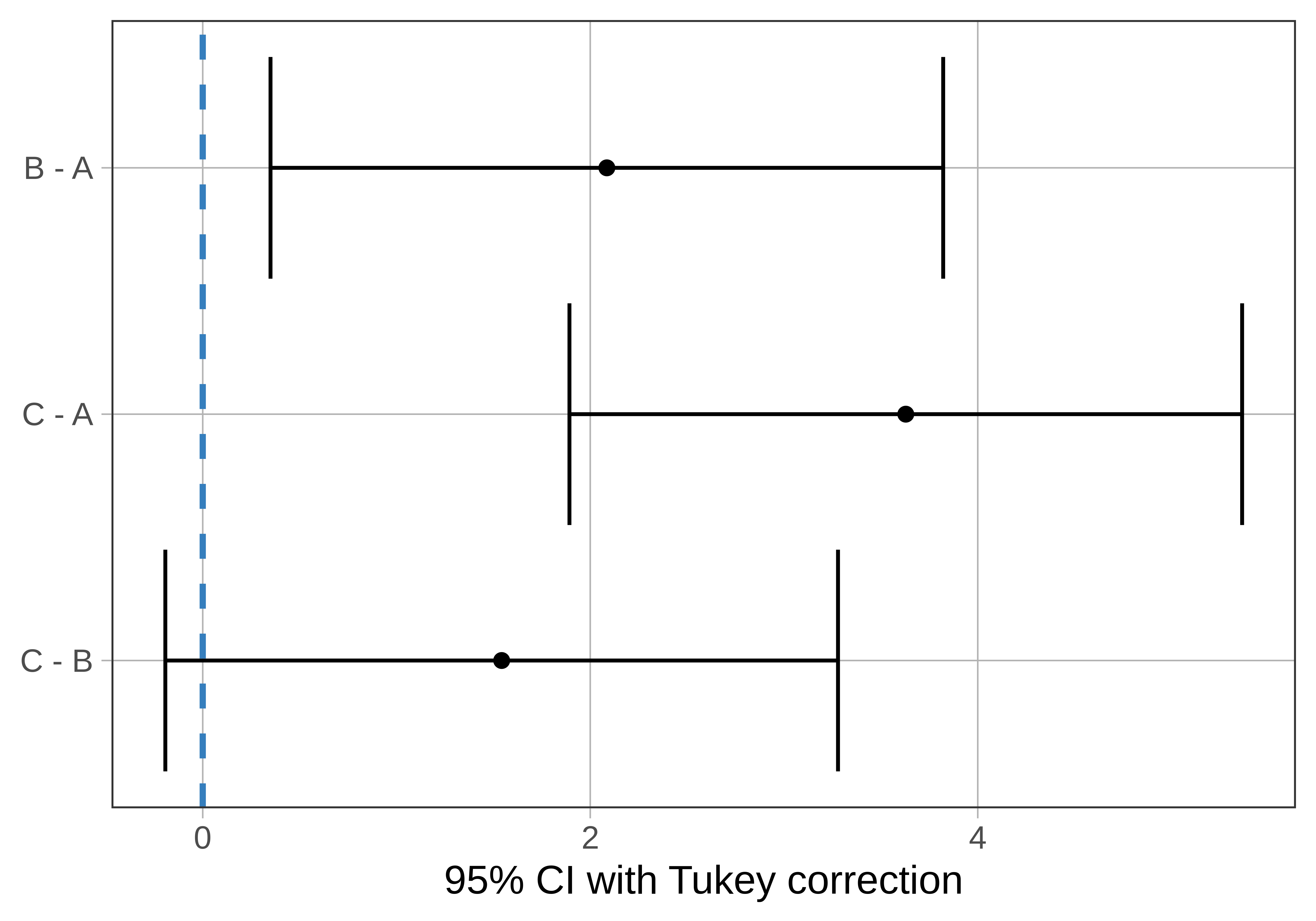
Notice that one of the 95% confidence intervals crosses the dotted line, which represents a pairwise difference of 0: C and B. But the other two confidence intervals (C - A and B - A) do not include 0. This means that we are not confident that the mean difference in the DGP for these pairs could be 0. We would conclude that game A is indeed different from both games B and C in the DGP.