8.9 Error and Inference from Models with Multiple Categorical Predictors

The ANOVA Table for the tip_percent ~ condition + gender Model

Let’s take a look at the ANOVA table to see how much error has been reduced (or, explained) by the multivariate model and how much each predictor uniquely contributes to this overall model.

Analysis of Variance Table (Type III SS)
 Model: tip_percent ~ condition + gender

                                    SS df       MS      F    PRE     p
 --------- --------------- | --------- -- -------- ------ ------ -----
     Model (error reduced) |  2534.538  2 1267.269 12.667 0.2275 .0000
 condition                 |    12.154  1   12.154  0.121 0.0014 .7283
    gender                 |  2531.353  1 2531.353 25.302 0.2273 .0000
     Error (from model)    |  8603.860 86  100.045                    
 --------- --------------- | --------- -- -------- ------ ------ -----
     Total (empty model)   | 11138.398 88  126.573   

We can represent this result in the Venn diagram below. gender overlaps quite a bit with tip_percent, which corresponds with its relatively large PRE of 0.2273. condition, on the other hand, reduces very little of the error in tips, with a PRE of 0.0014.

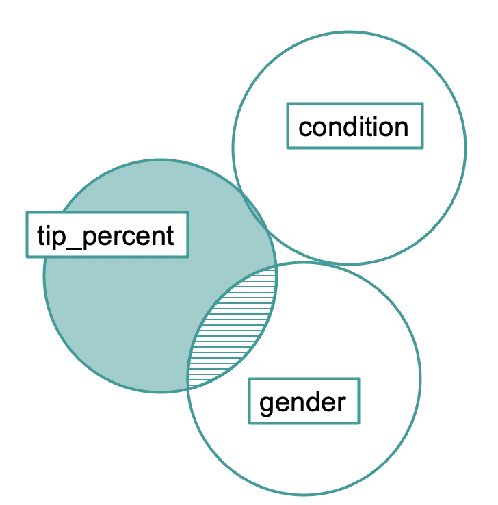
Notice that the condition variable overlaps hardly at all with gender in the Venn diagram, indicating very little relationship between the two predictor variables. By randomly assigning tables to both condition and gender, the researchers have ensured that there will be no relationship between the two predictor variables. Female servers are no more likely to be in the smiley face condition than males. This research design helps us get a better estimate of the independent effects of the two predictors.

Interpreting the p-values

The p-values in the ANOVA table can help us compare different possible models of the DGP.

Analysis of Variance Table (Type III SS)
 Model: tip_percent ~ condition + gender

                                    SS df       MS      F    PRE     p
 --------- --------------- | --------- -- -------- ------ ------ -----
     Model (error reduced) |  2534.538  2 1267.269 12.667 0.2275 .0000
 condition                 |    12.154  1   12.154  0.121 0.0014 .7283
    gender                 |  2531.353  1 2531.353 25.302 0.2273 .0000
     Error (from model)    |  8603.860 86  100.045                    
 --------- --------------- | --------- -- -------- ------ ------ -----
     Total (empty model)   | 11138.398 88  126.573   

The p-value for condition (.73) means that the F ratio for condition in the multivariate model could easily have been generated just by random chance, even if the true effect of condition in the DGP were actually equal to 0. We therefore would not reject the simple model (tip_percent ~ gender) being compared to the multivariate model.

The p-value for gender (.0001) implies a different story. It says that there is a less than .0001 chance that the F for gender would have resulted from a DGP in which the effect of gender is equal to 0. We can reject a model, therefore, that does not include gender (in this case, the model tip_percent ~ condition).

Selecting a Model of the DGP

Based on what we have learned from the ANOVA table, it seems reasonable to arrive at a final model of tip_percent ~ gender. Before finalizing our decision, we can compare the parameter estimates and ANOVA tables for the multivariate and gender models.

The two ANOVA tables look like this:

Multivariate Model: tip_percent ~ condition + gender

                                    SS df       MS      F    PRE     p
 --------- --------------- | --------- -- -------- ------ ------ -----
     Model (error reduced) |  2534.538  2 1267.269 12.667 0.2275 .0000
 condition                 |    12.154  1   12.154  0.121 0.0014 .7283
    gender                 |  2531.353  1 2531.353 25.302 0.2273 .0000
     Error (from model)    |  8603.860 86  100.045                    
 --------- --------------- | --------- -- -------- ------ ------ -----
     Total (empty model)   | 11138.398 88  126.573  

Gender Model: tip_percent ~ gender

Model: tip_percent ~ gender

                                SS df       MS      F    PRE     p
 ----- --------------- | --------- -- -------- ------ ------ -----
 Model (error reduced) |  2522.384  1 2522.384 25.470 0.2265 .0000
 Error (from model)    |  8616.014 87   99.035                    
 ----- --------------- | --------- -- -------- ------ ------ -----
 Total (empty model)   | 11138.398 88  126.573

When we look at the confidence intervals around the parameter estimates for gendermale (the change in prediction if the table had a male server), we see that they are similar between the single parameter model and the multivariate model (somewhere between -15 and -6.5).

Both models estimate that male servers will get lower tip percentages. The fact that the parameter estimates between the models don’t change very much reflects the fact that there is very little redundancy between condition and gender.