3.9 Error from the HomeSizeK Model
Regardless of model, error from the model (or residuals) are always calculated the same way for each data point:
\[residual=observed\ value - predicted\ value\]
For regression models, the predicted value of \(Y_i\) will be right on the regression line. Error, therefore, is calculated based on the vertical gap between a data point’s value on the Y axis (the outcome variable) and its predicted value based on the regression line.
Below we have depicted just 6 data points (in black) and their residuals (firebrick vertical lines) from the HomeSizeK model.
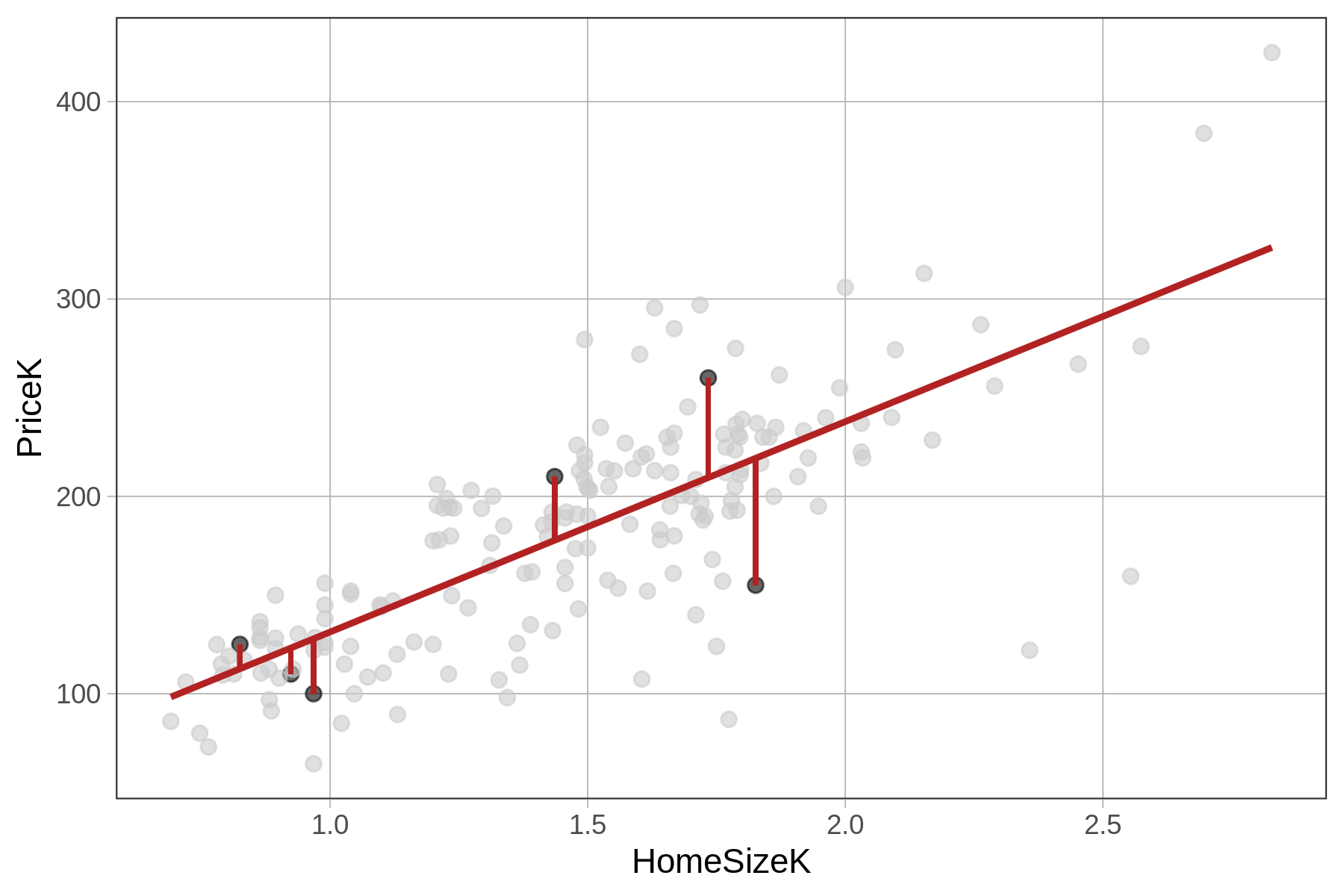
Note that a negative residual (shown below the regression line) means that the data (e.g., PriceK) was lower than the predicted price given the home’s size.
The residuals from the HomeSizeK model represent the variation in PriceK that is leftover after we take out the part that can be explained by HomeSizeK. As an example, take a particular house (highlighted in the plot below) that sold for $260K. The residual of 50 means that the house sold for $50K more than would have been predicted based on its size.
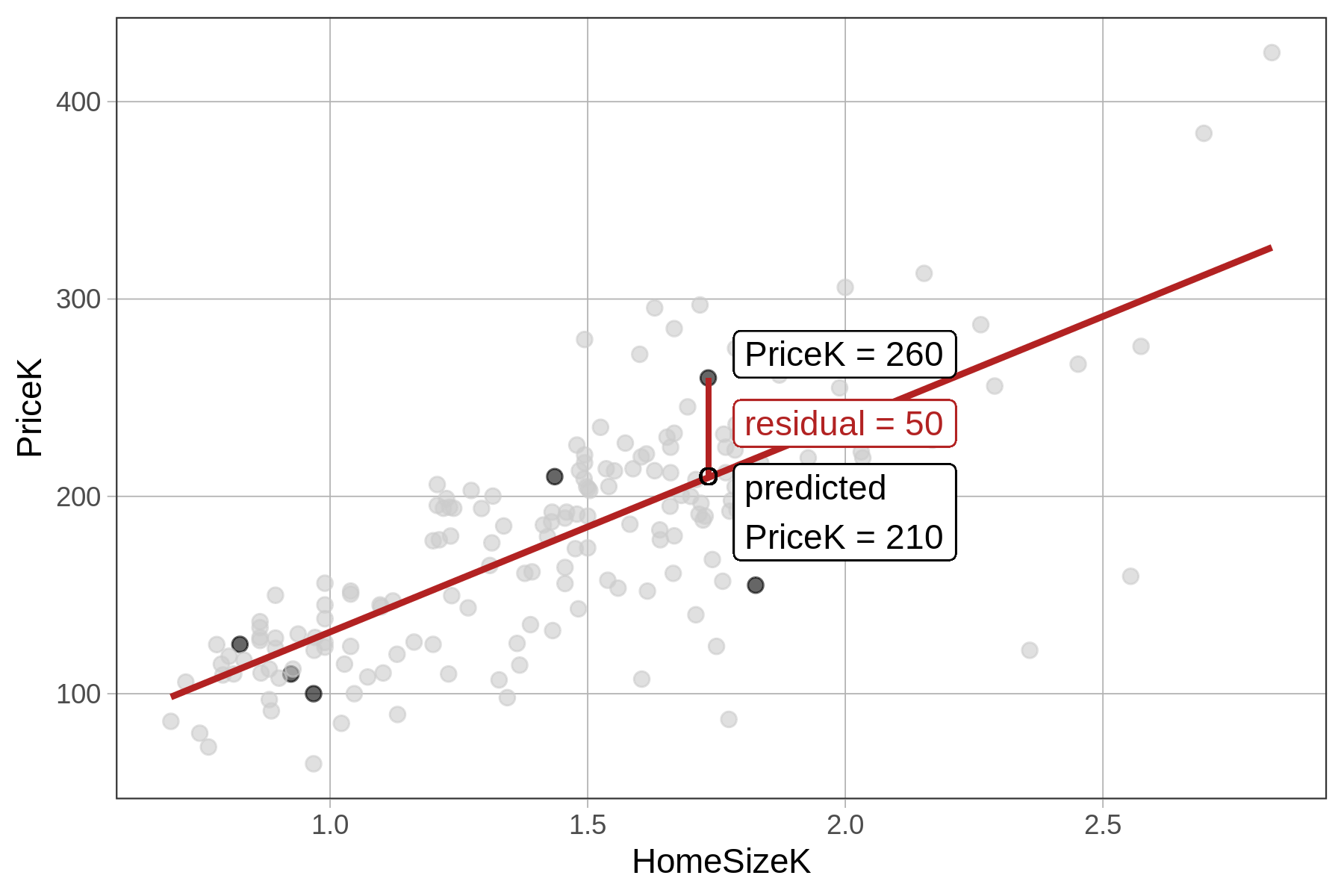
Another way we could say this is: Controlling for home size, this house sold for $50K more than expected. A positive residual indicates that a house is expensive for its size. A negative residual indicates that a house is cheap for its size (maybe prompting us to ask – “Hey! What’s wrong with it?”).
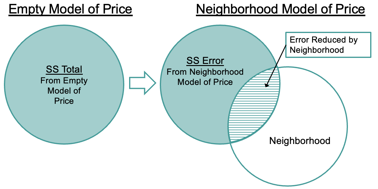
SS Error for the HomeSizeK Model
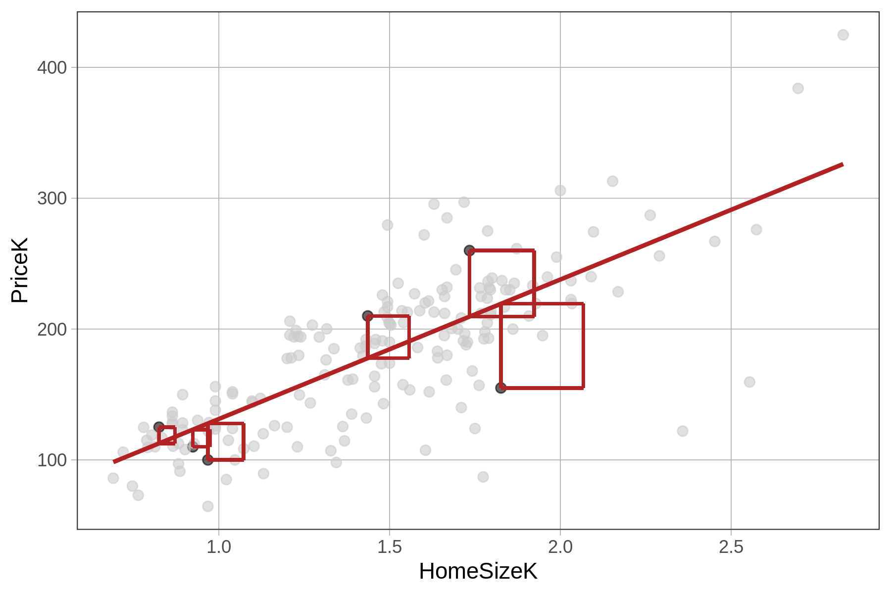
Just like for the Neighborhood model, the metric we use for quantifying total error from the HomeSizeK model is the sum of squared residuals from the model, or SS Error. The sum of squares is calculated from the residuals in the same way as it is for the Neighborhood model, by squaring and then summing the residuals (see figure below).
Using R to Compare SS for the HomeSizeK Model and the Empty Model
Just like we did with the Neighborhood model, we can use the resid() function to get the residuals from the HomeSizeK model. We can square them and sum them to get the SS Error from the model like this:
HomeSizeK_model <- lm(PriceK ~ HomeSizeK, data = Ames)
sum(resid(HomeSizeK_model)^2)
The code below will calculate SST from the empty model and SSE from the home size model. Run it to check your predictions about SSE.
require(coursekata)
# this calculates SST
empty_model <- lm(PriceK ~ NULL, data=Ames)
print("SST")
sum(resid(empty_model)^2)

# this calculates SSE
HomeSizeK_model <- lm(PriceK ~ HomeSizeK, data = Ames)
print("SSE")
sum(resid(HomeSizeK_model)^2)
# no test
ex() %>% check_error()[1] "SST"
633717.215434616
[1] "SSE"
258952.710665327Notice that the SST is the same as it was for the Neighborhood model: 633,717. This is because the empty model hasn’t changed, assuming that the same data points go into each analysis; SST is still based on residuals from the grand mean of PriceK. The SSE (258,952) is smaller than SST because the residuals are smaller (as represented in the figures above by shorter lines). Squaring and summing smaller residuals results in a smaller SSE. The total error has been reduced quite a bit by this regression model.
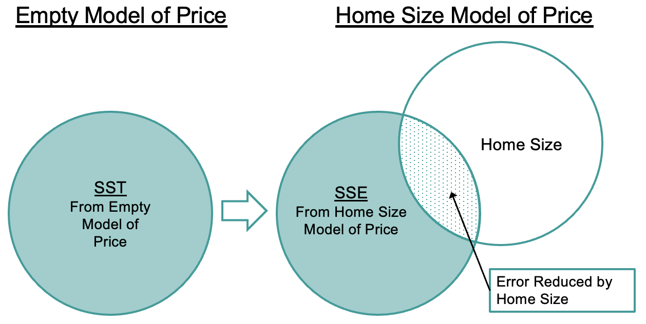
We’ve been talking about the SS Total and SS Error in relation to the HomeSizeK model. Let’s shift back to considering the Neighborhood model. Notice that in both models, we are partitioning SST into two parts: the part of SST that has been reduced by the model (which we will discuss more on the next page); and SSE, which is the amount of error still leftover after applying the model.