7.4 Interpreting the Parameter Estimates for a Multivariate Model

Using the Parameter Estimates to Make Predictions

We use the parameter estimates to make predictions in the same way as we did before, but this time we adjust our prediction based on two variables: what neighborhood a home is in (Neighborhood) and the amount of living space in the home (HomeSizeK).

Here is the best-fitting model that we found on the previous page:

\[\text{PriceK}_i = 177.25 + -66.22\text{NeighborhoodEastside}_i + 67.85\text{HomeSizeK}_i\]

We use the parameter estimates to make predictions from the multivariate model in the same way we did for single predictor models: each estimate (other than \(b_0\)) is multiplied by its corresponding variable (e.g., \(\text{NeighborhoodEastside}_i\) or \(\text{HomeSizeK}_i\)). Now let’s try to understand how the variables in the multivariate model are coded in order to generate predictions.

The model, which is a function, generates a predicted home price (in 1000s of dollars) by starting with the intercept (\(b_0\), which is 177.25), then subtracting 66.22 if the home is in Eastside, and then adding on 67.85 for each 1000 square feet of living space in the home.

Interpreting the Parameter Estimates

So far, the parameter estimates from the multivariate model might seem pretty similar to the parameter estimates from single-predictor models. But the estimates themselves are not exactly the same. This is because the estimates have a slightly different meaning in the multivariate model than they do in the single-predictor models.

In the two-predictor model, each home’s value is assumed to be a function of both Neighborhood and HomeSizeK. But these two things are not independent of each other. To help explain what we mean, take a look at the faceted histogram below. You’ve seen it before, but this time we colored two of the homes red.

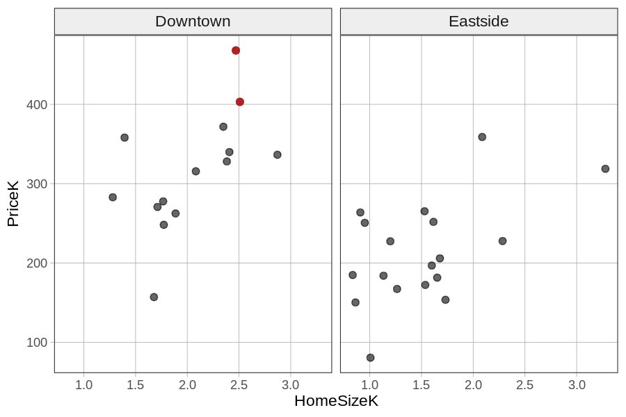
These two homes happen to be the two most expensive homes in the Smallville data frame. But what makes them expensive? Is it the neighborhood they are in, or is it that they also are among the larger homes in the data frame? The answer is that it probably is a little of both.

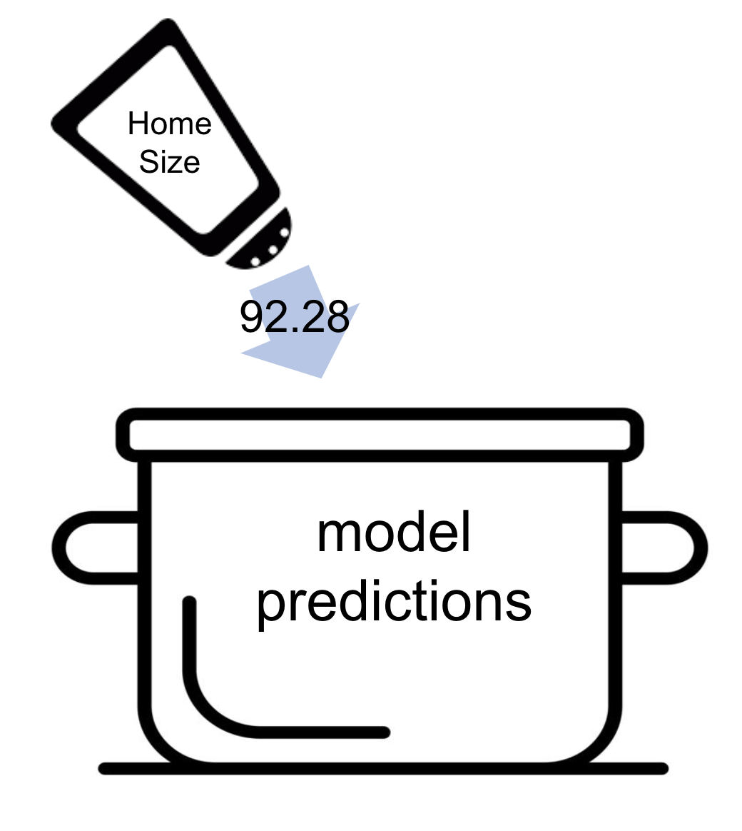
Because the two variables are related to each other (i.e., Downtown tends to have larger houses than Eastside), the parameter estimate for the single-predictor HomeSizeK model (\(b_1 = 92.28\)) includes a little bit of the adjustment in predicted price that might actually be due to Neighborhood.

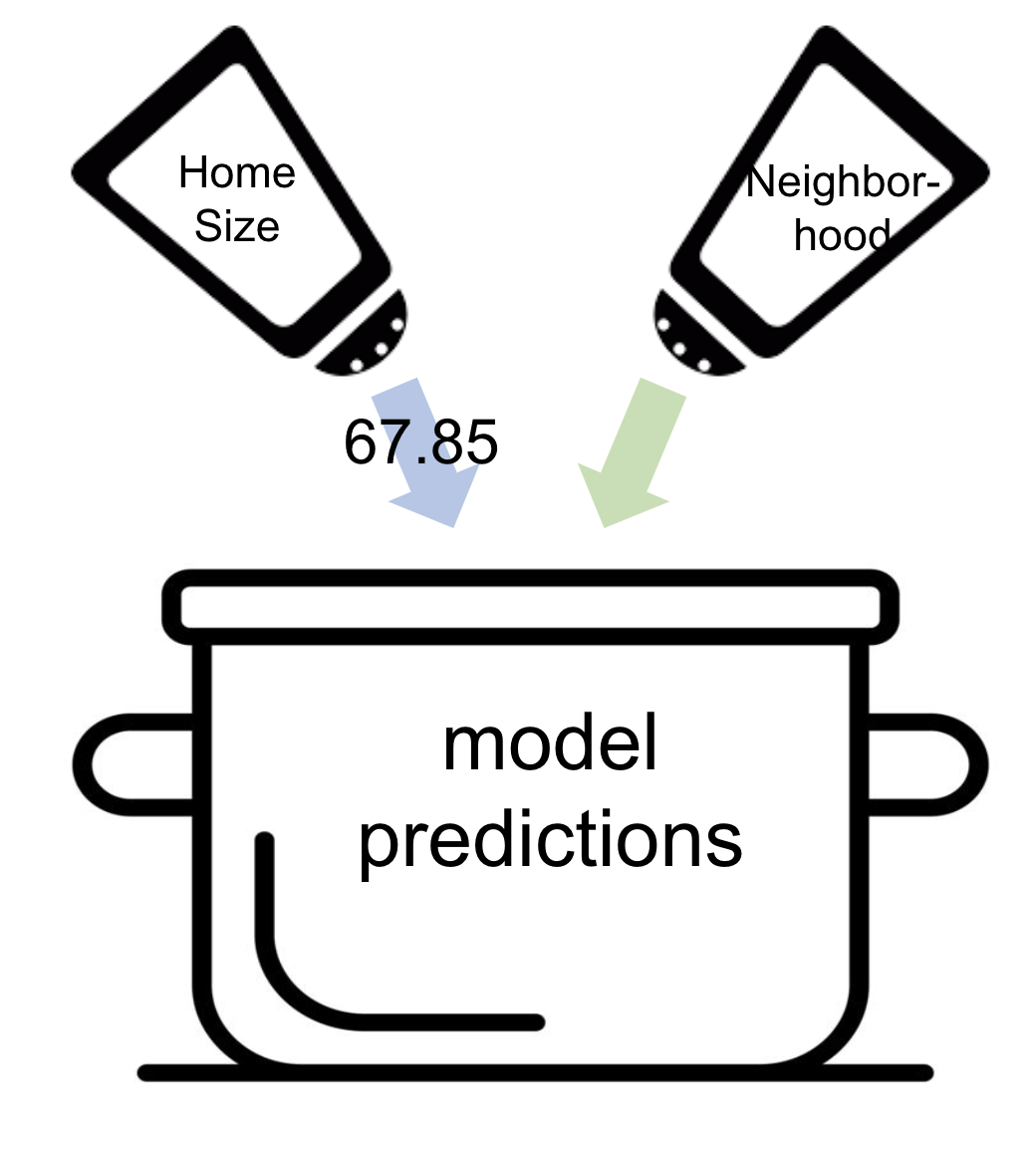
When we add Neighborhood into the model (making a multivariate model), R takes some of that adjustment that was originally attributed completely to HomeSizeK and attributes it to Neighborhood. Take a look at the \(b\) in front of \(\text{HomeSizeK}_i\) in the models below:

HomeSizeK Model: \(\text{PriceK}_i = 97.47 + \colorbox{yellow}{92.28}\text{HomeSizeK}_i\)

Multivariate Model: \(\text{PriceK}_i = 177.25 + -66.22\text{NeighborhoodEastside}_i + \colorbox{yellow}{67.85}\text{HomeSizeK}_i\)

Because the parameter estimate for HomeSizeK in the multivariate model knows that Neighborhood is also in the model, it is a little less extreme in the multivariate model than in the single-predictor model.

To return to our cooking analogy, in the single-predictor HomeSizeK model, home size did all the work in seasoning the predictions. But in the model with both HomeSizeK and Neighborhood, neighborhood will add a little bit of the seasoning that was previously added by home size. Because parameter estimates moderate the contributions of each variable, they are sometimes called “weights”.

In the single-predictor model, the \(b\)s are called regression coefficients: they tell us how much to add to the prediction for each 1 unit increase in X. In multiple-predictor models we will call the \(b\)s partial regression coefficients because how much the model adds depends on the other explanatory variables in the model. Another way to say this is that the \(b\) tells us the effect of a variable “controlling for” all the other variables in the model.