7.6 Using Residuals and Sums of Squares to Measure Error Around the Multivariate Model

In most respects, concepts developed for the single-predictor models will apply to the multi-predictor models. In all cases, the model generates a predicted value on the outcome variable for each observation in the data frame. Subtracting the model prediction from the observed value will give us a residual, which tells us how far off the model prediction is (positive or negative) for each observation.

If we square and then total up all the residuals we will get the SS Error for the model, which gives us a sense of how well the model fits the data. Using this SS Error, we can then compare the multi-predictor model to other models, starting with the empty model. To assess how well a model fits the data we will continually ask: How much does one model reduce error over another?

Residuals From the Multivariate Model

Error from the multivariate model is calculated in exactly the same way as for the other models we have considered. Each model generates a prediction for each data point, and because the predictions are usually wrong, we can use the difference between the predicted and actual values to arrive at a residual for each observation.

Let’s look again at the scatterplot of PriceK by HomeSizeK, with each neighborhood represented in a different color. Now let’s zero in on one particular home in Downtown that sold for a little over $400K (the solid teal dot).

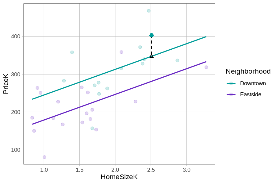
Using the predict() and resid() functions, we can generate and save the multivariate model’s predictions and residuals in the Smallville data frame.

Smallville$multi_predict <- predict(multi_model)
Smallville$multi_resid <- resid(multi_model)

Here is the print out of the prediction and residual for the house represented by the teal dot (above):

  PriceK multi_predict multi_resid
 403.101      347.4862     55.6148

The actual price of the home is equal to the prediction + the residual (i.e., 403.101 = 347.4862 + 55.6148). Because the data point is higher than the model prediction, the residual is positive. Connecting back to DATA = MODEL + ERROR, you can see which part of the equation below represents the actual price of this home (403K), the model’s prediction (347K), and the residual (56K).

\[\underbrace{\text{PriceK}_i}_{\mbox{403K}} = \underbrace{b_0 + b_1\text{NeighborhoodEastside}_i + b_2\text{HomeSizeK}_i}_{\mbox{347K}} + \underbrace{e_i}_{\mbox{56K}}\]

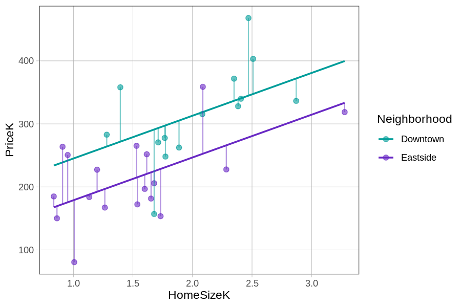
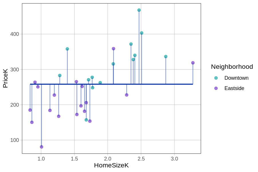
We will see this pattern (DATA = MODEL + ERROR) no matter how complex or simple the model is. All models produce predictions and those predictions have some residual error. Below we show how the residuals for the same 6 data points depend on what model (multivariate versus empty model) is used to make the predictions.

Residuals from the Multivariate Model \(Y_i = b_0 + b_1X_{1i} + b_2X_{2i} + e_i\)	Residuals from the Empty Model \(Y_i = b_0 + e_i\)

Using the ANOVA Table to Compare the Multivariate Model to the Empty Model

We might believe our multivariate model is better, but how much better is it? To begin to answer this question, let’s start by comparing the sum of squared error from our new model to the error from the empty model.

We previously used the supernova() function to generate ANOVA tables that contain the SSs useful for comparing models. In the code block below we have fit the multivariate model and saved it as multi_model. Add code to generate the supernova() output for our model.

Analysis of Variance Table (Type III SS)
 Model: PriceK ~ Neighborhood + HomeSizeK

                                        SS df        MS      F    PRE     p
 ------------ --------------- | ---------- -- --------- ------ ------ -----
        Model (error reduced) | 124403.028  2 62201.514 17.216 0.5428 .0000
 Neighborhood                 |  27758.259  1 27758.259  7.683 0.2094 .0096
    HomeSizeK                 |  42003.677  1 42003.677 11.626 0.2862 .0019
        Error (from model)    | 104774.465 29  3612.913                    
 ------------ --------------- | ---------- -- --------- ------ ------ -----
        Total (empty model)   | 229177.493 31  7392.822                   

You may notice right away that this ANOVA table has more rows than the one for either the neighborhood model or the home size model. Don’t worry about these new rows for now – just look for SS Total, SS Error, and SS Model; these have the same meaning as in the single-predictor models.

SS Total

As before, SS Total = SS Model + SS Error (which is the sum of squares version of DATA = MODEL + ERROR). Use the code block below to verify (with simple arithmetic) that SS Model + SS Error really does equal SS Total using the highlighted numbers in the ANOVA table above.

SS Total (the bottom row of the ANOVA table) tells us how much total variation, measured in sum of squares, there is in the outcome variable. You can see that SS Total is 229,177.

SS Total is all about the outcome variable, in this case PriceK. It is based on squaring and then summing residuals from the empty model. No matter which predictor variables you add to your model, SS Total, the last row in the ANOVA table, is always the same as long as the outcome variable is the same.The empty model of an outcome variable does not depend on any predictor variables.

SS Error and SS Model

SS Error is the generic name we give to the sum of the squared residuals leftover after fitting a complex model (by “complex” we just mean a model that is more complex than the empty model). Because SS Total = SS Model + SS Error, the lower SS Error is, the higher SS Model will be, meaning that more of the variation has been explained by the model, which is the same as saying that more of the error has been reduced by the model.

We can apply the concepts of SS Model and SS Error to any model, from those with just a single predictor all the way to those with many predictors.