10.7 Visually Comparing the Interaction Model to the Additive Model with Two Categorical Predictors
In the previous chapter we fit the additive model to this same data. Whereas the additive model was a three parameter model (\(b_0\), \(b_1\), and \(b_2\)) the interaction model requires us to estimate one additional parameter (\(b_3\)). Let’s take a brief look back at what the additive model looks like, and see what we have “bought” with this extra parameter.
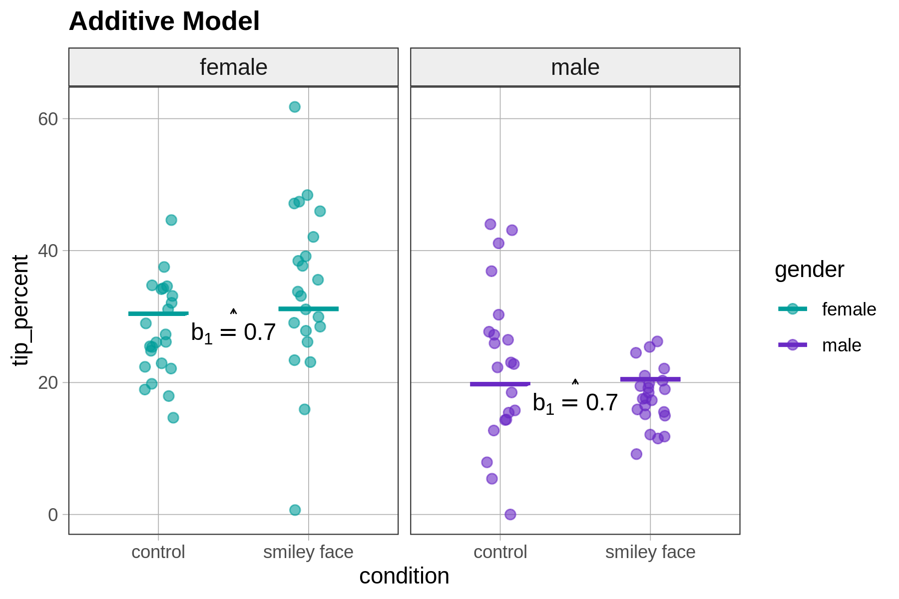
In the table below we’ve put two jitter plots. On the right is the one we have just been discussing, with the interaction model predictions overlaid. On the left is the same jitter plot, with the same data, but this time with the predictions of the additive model.
| Additive Model | Interaction Model |
|---|---|
|
|
|
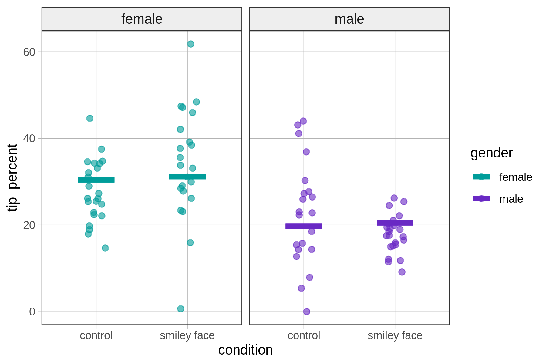
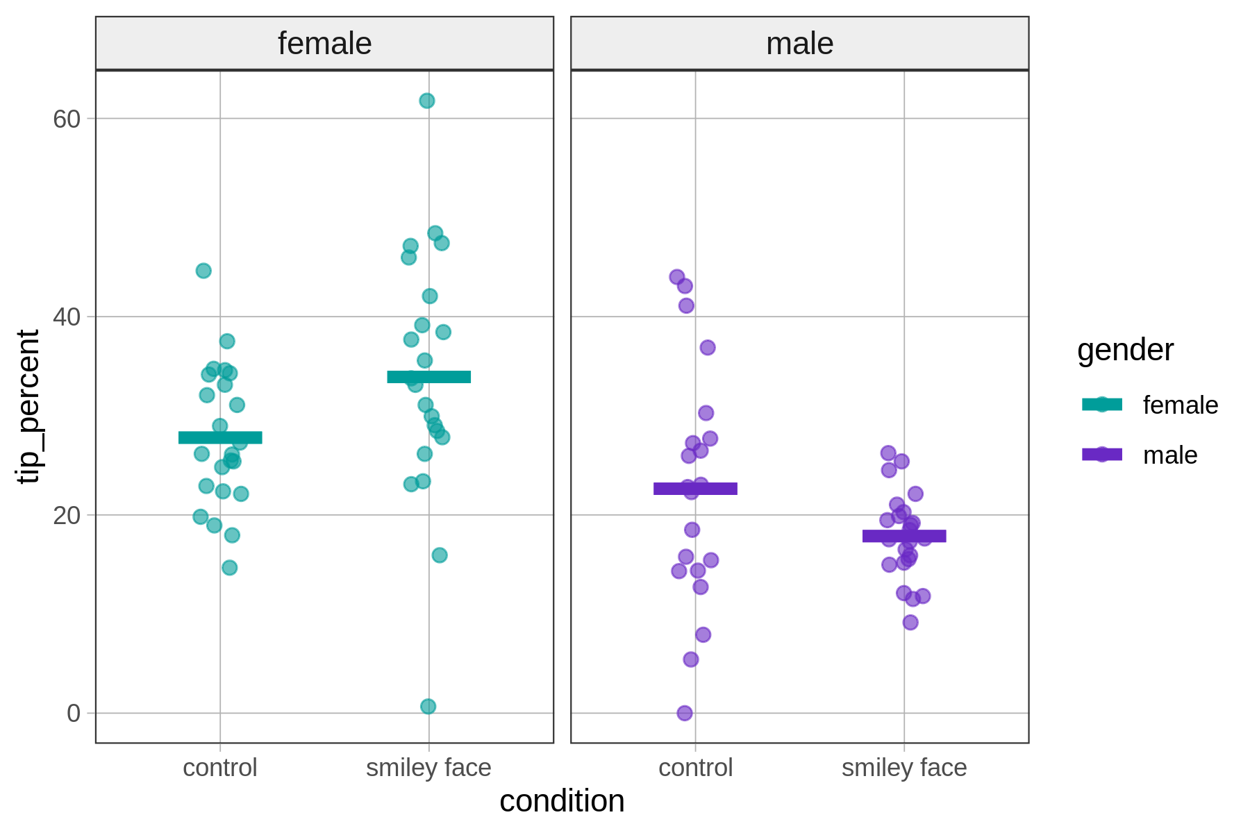
Whereas the size of the effect of condition on tip percent is free to differ for females and males in the interaction model, that freedom is not there in the additive model. When we ask R to fit the additive model we are telling it to assume that the effect of condition is the same for both genders, and that the effect of gender is the same regardless of condition. These constraints lead to very different best-fitting parameter estimates:
Additive model:
\(30.42 + 0.74\text{conditionsmiley} + -10.67\text{gendermale}\)
Interaction model:
\(27.79 + 6.12\text{conditionsmiley} + -5.16\text{gendermale} + -10.9\text{conditionsmiley}*\text{gendermale}\)
In the additive model, the predicted effect of being in the smiley face condition is small and exactly the same for females as it is for males. Thus, for both females and males, the model adds the same amount (\(b_1\), or $0.74) to go from control to smiley face. Although this is the best-fitting additive model, the best model may not be additive.
The interaction model, by contrast, adds one additional parameter (\(b_3\)), which allows it to make a unique prediction for each of the four groups. Thus the effect of condition can be different for females and males. For females, therefore, the model adds \(b_1\) to go from control to smiley face, whereas for males it adds \(b_1+b_3\).
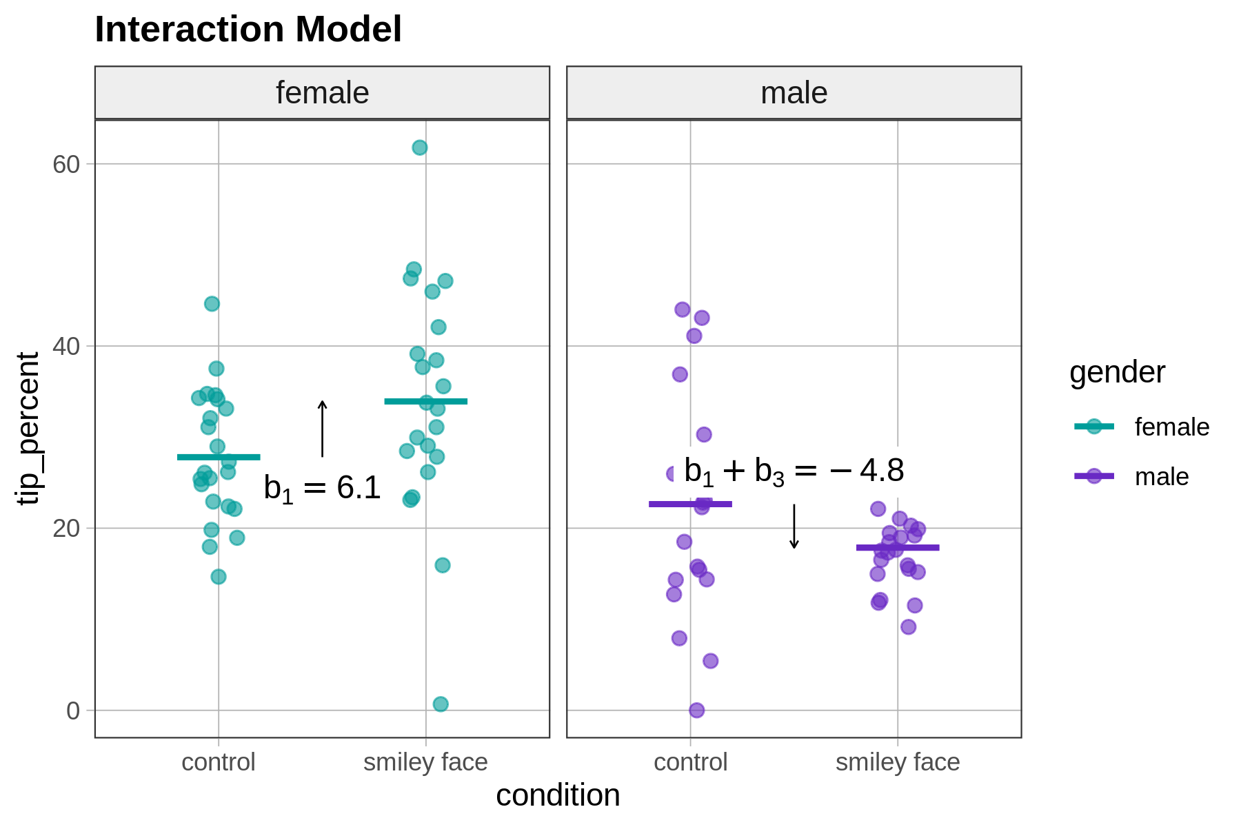
In the tipping study data, this seems like a good idea: females actually get a boost in tips when they go from control to smiley face, whereas males see their tips go down. From what we can see in the graph, the interaction model appears to be a better fit to the data.
By adding one more parameter, the effect of condition no longer needs to apply equally to females and males, and the effect of gender does not need to apply equally across conditions.
It’s useful to connect the visual comparison of the additive and interaction models with the GLM function used to predict the tips for each of the four groups. As you can see in the table below, the only difference in prediction functions for the two models is in the cell for male servers who drew smiley faces.
| Additive Model Predictions | ||||
|---|---|---|---|---|
| \(\text{tip_percent} = b_0 + b_1\text{conditionsmiley} + b_2\text{gendermale}\) | ||||
| gender | 0 - female | 1 - male | ||
| condition | 0 - control | 1 - smiley face | 0 - control | 1 - smiley face |
| prediction | \(b_0\) | \(b_0+b_1\) | \(b_0+b_2\) | \(b_0+b_1+b_2\) |
| Interaction Model Predictions | ||||
| \(\text{tip_percent} = b_0 + b_1\text{conditionsmiley} + b_2\text{gendermale}+b_3\text{conditionsmiley}*\text{gendermale}\) | ||||
| gender | 0 - female | 1 - male | ||
| condition | 0 - control | 1 - smiley face | 0 - control | 1 - smiley face |
| prediction | \(b_0\) | \(b_0+b_1\) | \(b_0+b_2\) | \(b_0+b_1+b_2+b_3\) |
In both models, we start with \(b_0\), which is the prediction for females in the control condition and add \(b_1\) to that if a table is in the smiley face condition, and \(b_2\) if the server is male.
If a table is both in the smiley face condition and has a male server, the additive and interaction models diverge. In the additive model, we simply add \(b_1\) and \(b_2\). In the interaction model, we add \(b_3\) as well.