9.4 Interpreting Parameter Estimates for the Interaction Model

Let’s take a moment to connect the interaction model we’ve been developing to the basic idea DATA = MODEL + ERROR.

Using lm() to Fit a Model with an Interaction Term

In general, interaction terms are represented as the product of two explanatory variables (e.g., condition*base_anxiety). Fitting an interaction model in R is as simple as adding in this code to the additive model, like this:

lm(later_anxiety ~ condition + base_anxiety + condition*base_anxiety, data = er)

Use the code window below to fit the interaction model of later_anxiety. Save the model as interaction_model, and add some code to print out the model estimates.

Here are the model estimates for the interaction_model:

Call:
lm(formula = later_anxiety ~ condition * base_anxiety, data = er)

Coefficients:
              (Intercept)               conditionDog  
                  -0.3506                    -0.6388  
             base_anxiety  conditionDog:base_anxiety  
                   0.9437                    -0.2285

Whenever an interaction term (e.g., condition*base_anxiety) is included in a model, the individual variables that make up the interaction (e.g., condition and base_anxiety) must also be included. Because these lower-level terms are always included, lm() provides a shortcut for specifying an interaction model. If you write

lm(later_anxiety ~ condition*base_anxiety, data = er)

R will assume you want condition and base_anxiety in the model as well. Try it in the code window above; you’ll see that it produces the same output.

Graphing the Interaction Model

Now that we have fit the interaction model, we can add it onto a scatterplot or jitter plot using the gf_model() function. Add the interaction model to the plot in the code window below.

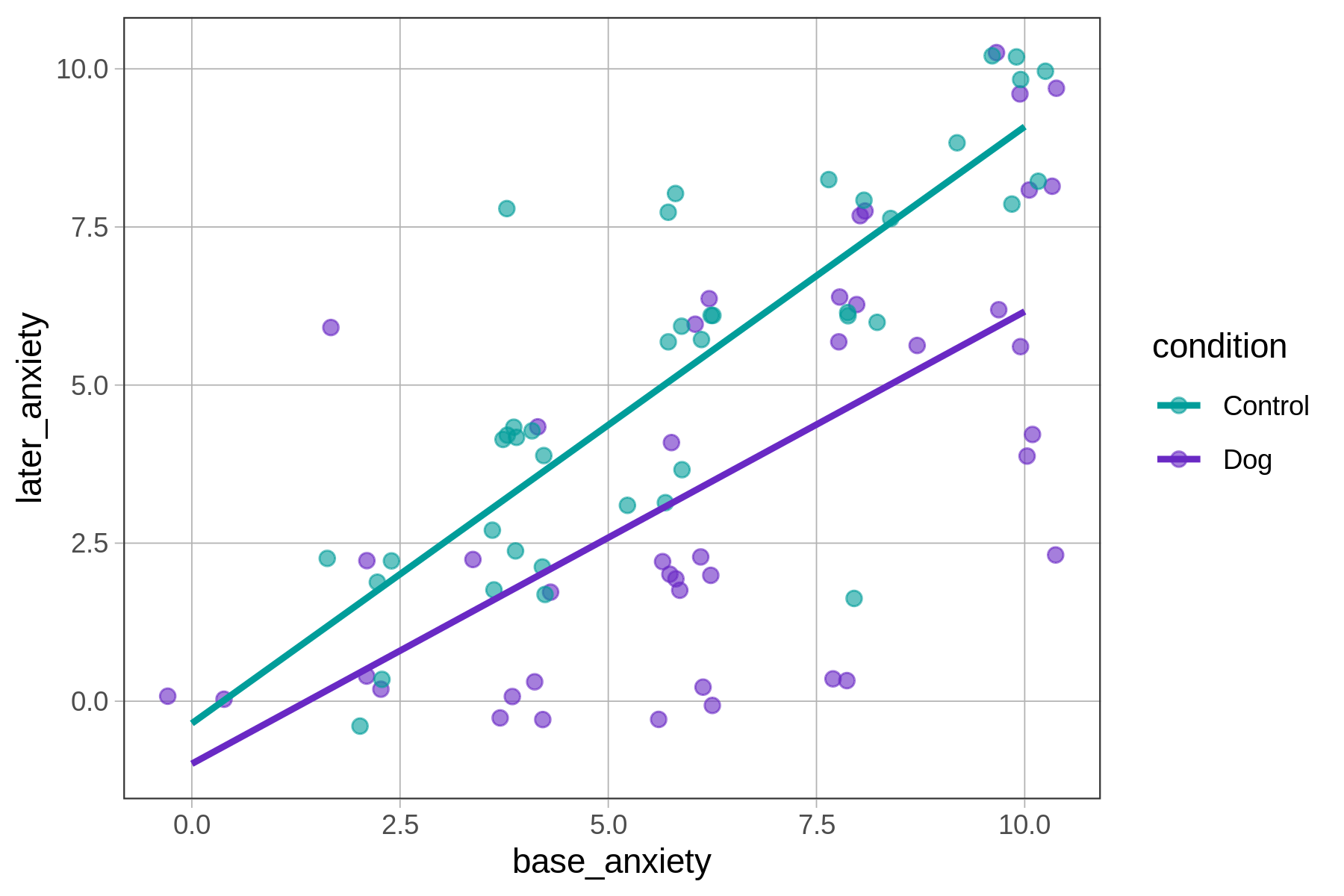
The best fitting interaction model is shown as two non-parallel lines, each with their own y-intercept and slope. The lines represent all the possible predictions of this model given the different values of base_anxiety and condition. Let’s dig into those predictions.

Generating Predictions from the Interaction Model

Like all statistical models, interaction models are functions that will generate a predicted score on the outcome variable (in this case later_anxiety) for each observation in the data frame.

In R, we can use the predict() function to generate predictions for all the observations we have in our er data. In the code window below, create and save a new variable in the er data frame called interaction_predict. Then we’ll print out the first six rows of the data frame to see a few predictions.

 later_anxiety base_anxiety condition interaction_predict
          <dbl>        <dbl> <chr>                   <dbl>
1             2            3 Dog                      1.16
2             9            9 Control                  8.14
3             3            5 Control                  4.37
4             8            8 Dog                      4.73
5             0            4 Dog                      1.87
6             2            2 Control                  1.54

As expected, the interaction model produces a prediction for later_anxiety for each patient based on their base anxiety and condition. In the graph below, we show the actual and predicted later_anxiety for these first six patients as solid dots and empty dots, respectively.

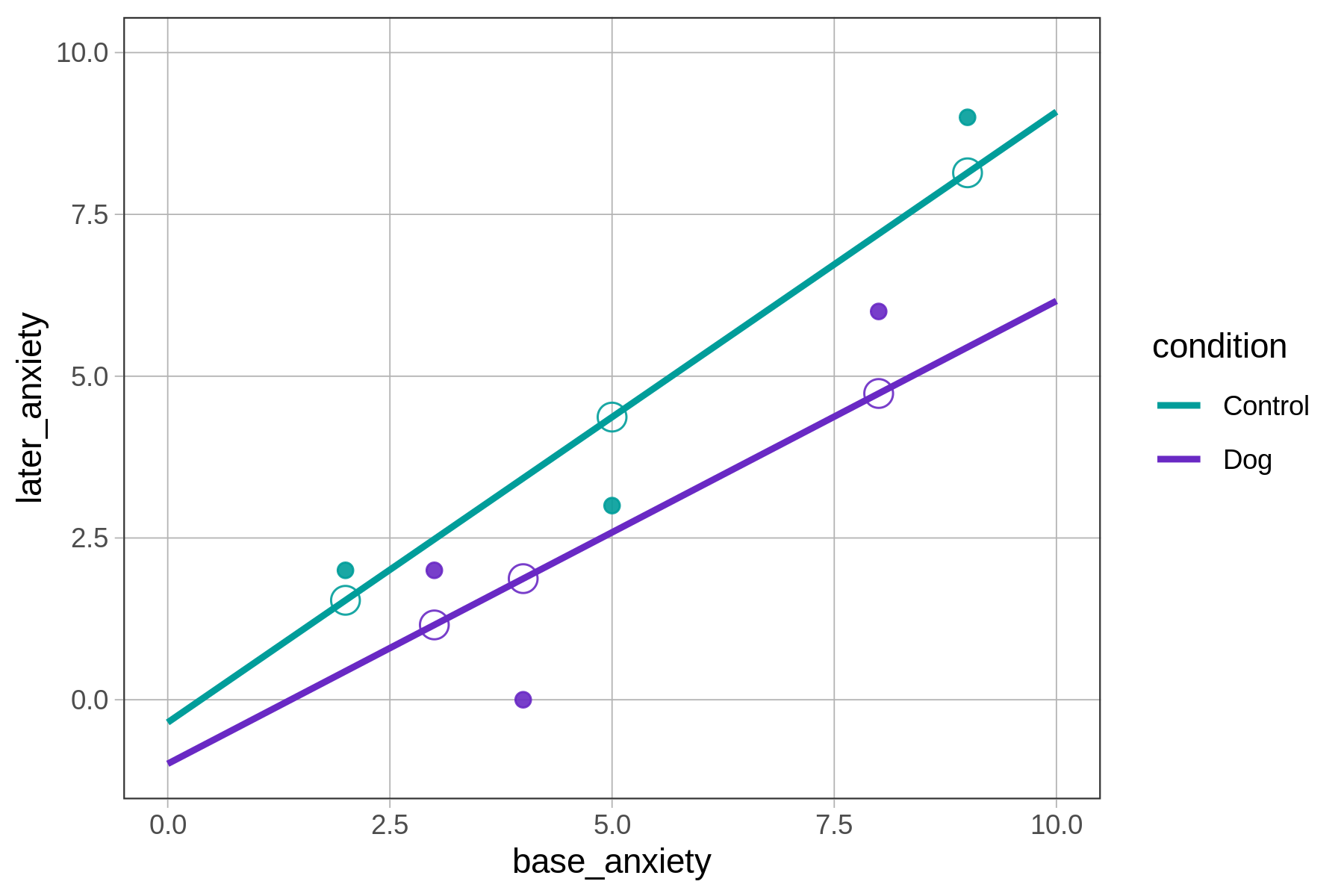
Notice that regardless of where the data points fall, predictions for patients in the control group all fall on the green line, whereas those for the dog group all fall on the purple line. This is no accident: these regression lines are the models from which the predictions are made.

Slopes, Y-Intercepts, and Parameter Estimates for Interaction Models

We’ve figured out what the parameter estimates (\(b\)s) mean in theory. The interaction model we have been exploring can be represented as two lines, each with its own slope and y-intercept. How do we use the parameter estimates to determine the slopes and intercepts of these two lines? Fitting our interaction model of later_anxiety produced the following parameter estimates:

Call:
lm(formula = later_anxiety ~ condition * base_anxiety, data = er)

Coefficients:
              (Intercept)               conditionDog  
                  -0.3506                    -0.6388  
             base_anxiety  conditionDog:base_anxiety  
                   0.9437                    -0.2285

We can replace the \(b\)s in the model with these estimates, like this:

\[\text{later}_i \hspace{6pt}=\hspace{6pt} b_0 \hspace{6pt}+\hspace{6pt} b_1\text{Dog}_i \hspace{6pt}+\hspace{6pt} b_2\text{base}_i \hspace{6pt}+\hspace{6pt} b_3\text{Dog}_i*\text{base}_i \hspace{6pt}+\hspace{6pt} e_i\]

\[\text{later}_i = -0.35 + -0.64\text{Dog}_i + 0.94\text{base}_i + -0.23\text{Dog}_i*\text{base}_i + e_i\]

Consider the table we made earlier.

condition	y-intercept	slope
Control	\(b_0\)	\(b_2\)
Dog	\(b_0 + b_1\)	\(b_2 + b_3\)

The y-intercepts and slopes are visible in the visual representation of the model predictions below.

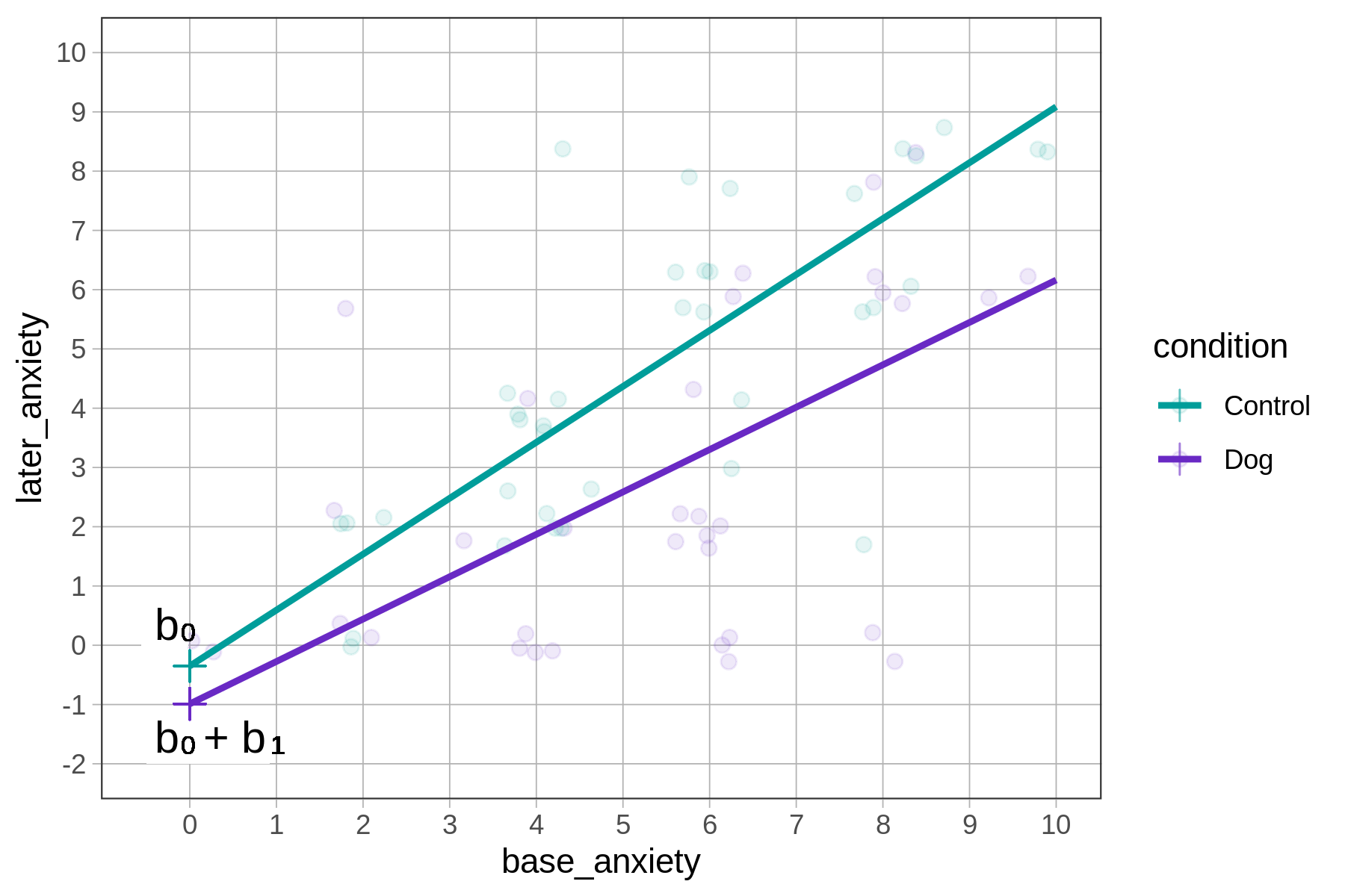
The control line’s y-intercept is a little bit negative (below the 0 mark on the y-axis); indeed, the best-fitting estimate for \(b_0 = -0.35\).

Here is the best-fitting interaction model again. Now let’s turn our attention to \(b_2\) and \(b_3\): \[\text{later}_i = -0.35 + -0.64\text{Dog}_i + \colorbox{yellow}{0.94}\text{base}_i + \colorbox{yellow}{-0.23}\text{Dog}_i*\text{base}_i + e_i\]

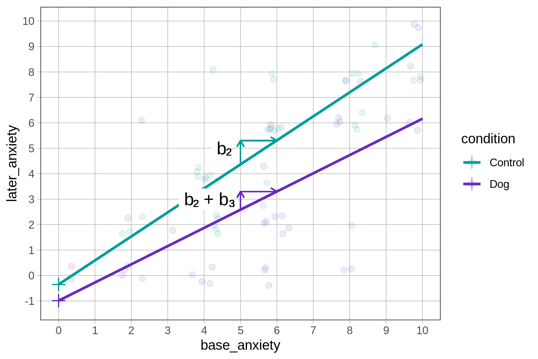
The slope of the dog predictions is slightly smaller (\(b_2 + b_3 = 0.94 - 0.23 = 0.71\)) than the slope of the control predictions (\(b_2 = 0.94\)).

As with all multivariate models, the best-fitting parameter estimate for one variable will differ depending on which other variables are included in the model. In this case, the estimates for \(b_0\), \(b_1\), and \(b_2\) would be different if the interaction term (\(b_3\text{Dog}_i*\text{base}_i\)) were not included in the model.