9.2 Additive versus Non-Additive Models
What makes a model additive?
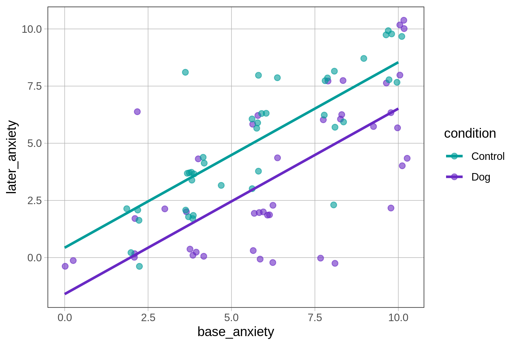
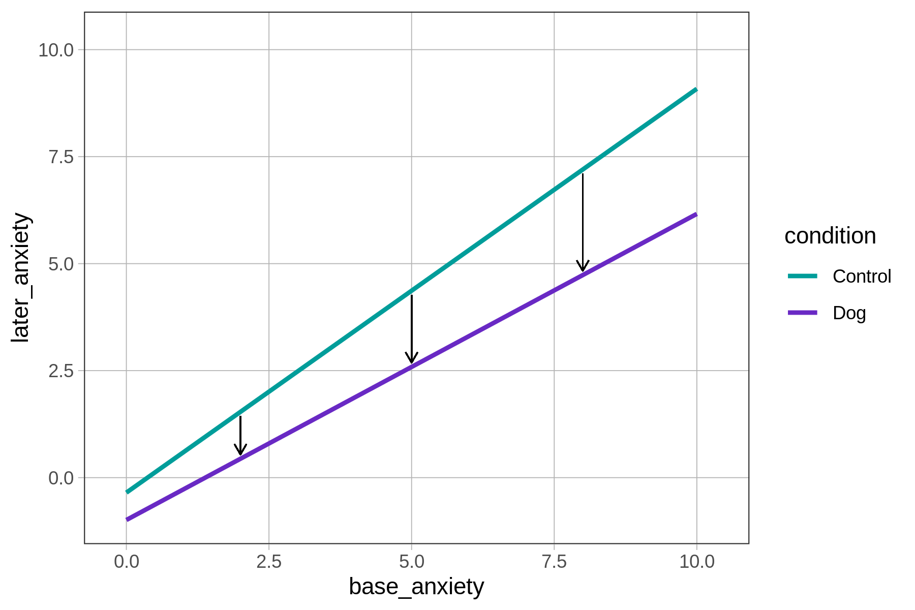
In the plot above, the data are represented by dots (each dot represents a person). The additive model is represented by the two regression lines, one for each of the two conditions (Dog and Control). The lines represent the model predictions for later_anxiety based on both condition and base_anxiety.
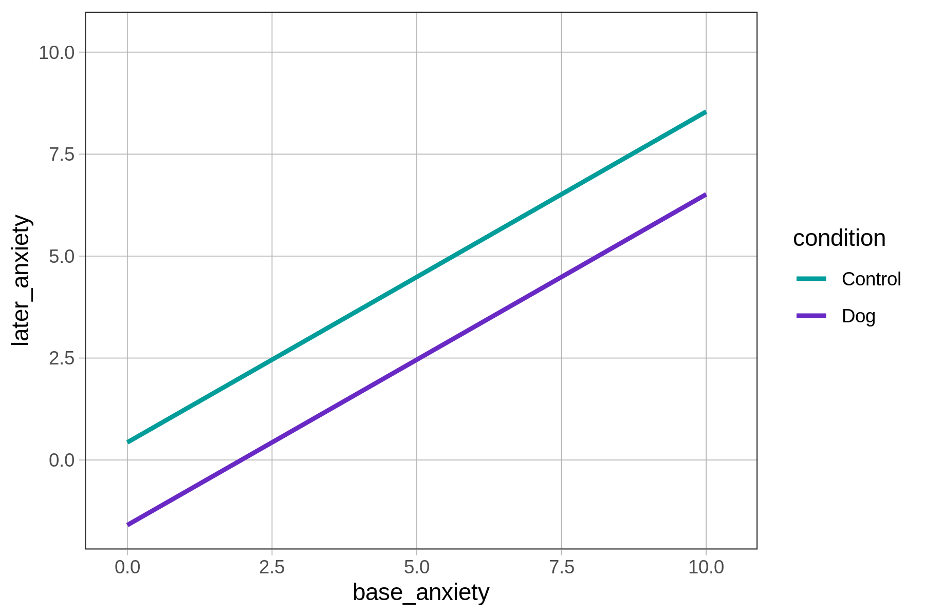
What makes this model additive can be seen in the graph: the two regression lines are parallel to each other. In a non-additive model, by contrast, the two lines would not be parallel (as shown in the figure below).
| Additive Model | Non-Additive Model |
|---|---|
|
|
|
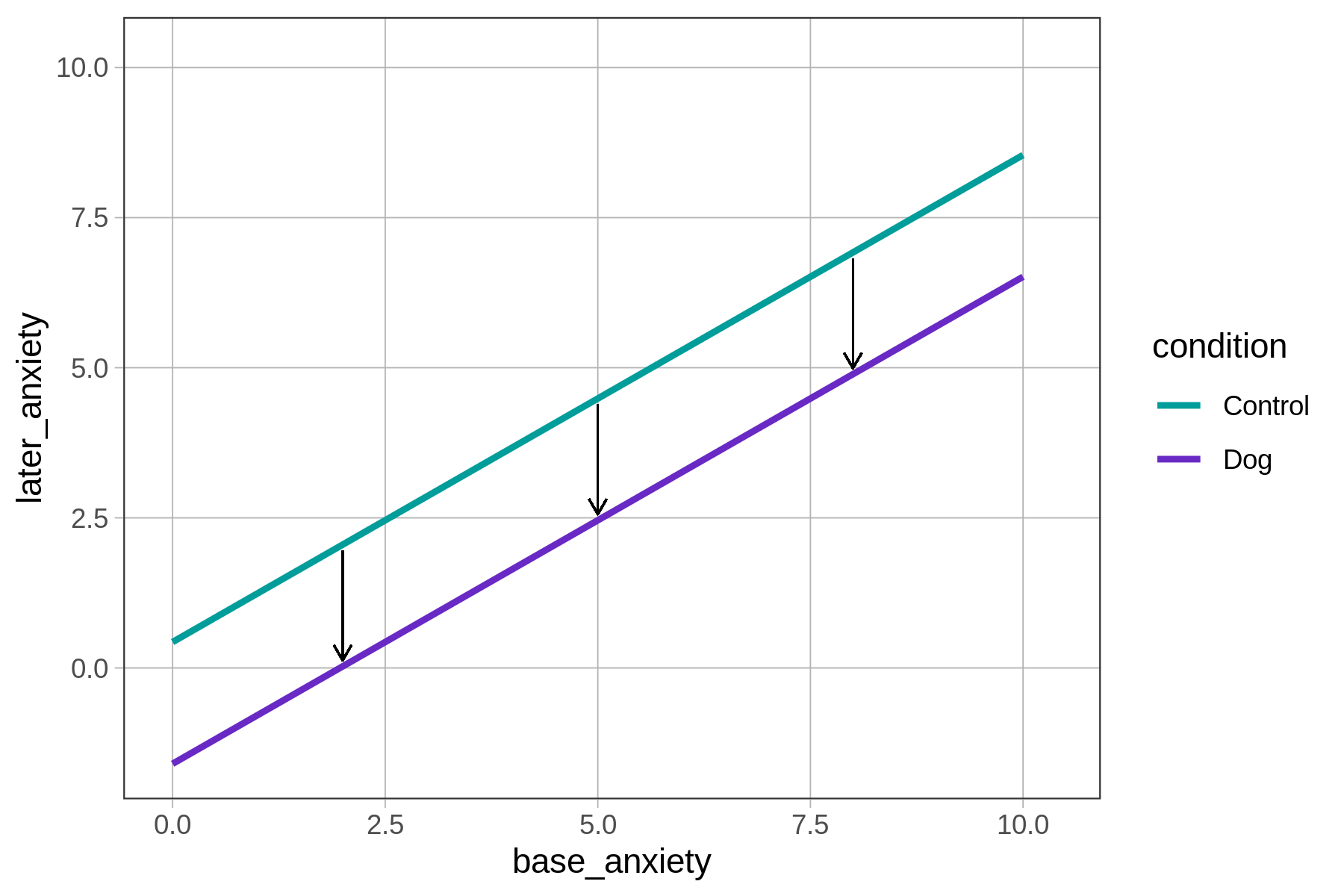
In the additive model, the predicted effect of condition on later_anxiety is the same, regardless of patients’ base_anxiety on arriving at the ER. No matter the base anxiety (e.g., 2, 5, 8), having a therapy dog results in a roughly 2-point reduction in later anxiety (shown by the vertical black lines above), which corresponds to the lm() function’s parameter estimate for conditionDog of -2.03.
Likewise, each additional point of base anxiety has the same effect on later anxiety regardless of which group a patient is in, which is another way of saying that the slopes of the two regression lines are the same: 0.81.
The parallel lines show that the difference between the dog and control groups is constant across all levels of base anxiety. Models are additive when the effect of one predictor variable on an outcome does not change based on values of a second predictor variable.
By writing the R code lm(later_anxiety ~ condition + base_anxiety, data = er) we are telling R to fit an additive model to the data. The additivity (you can think of it as parallelism) is a characteristic of the model; it may or may not be true of the data or of the DGP.
The Additive Model in GLM Notation
The additivity of the model is also represented in the GLM equation:
\[\text{later}_i=b_0+b_1\text{Dog}_i+b_2\text{base}_i\]
(Note we’ve abbreviated \(\text{later_anxiety}\) and \(\text{base_anxiety}\) into \(\text{later}\) and \(\text{base}\) to make the equations look a little shorter. We’ve similarly shortened the dummy variable \(\text{conditionDog}\) to \(\text{Dog}\). \(\text{Dog}\) is coded 1 if the patient was in the dog therapy condition, 0 if not.)
Notice that there is a part of this equation that represents the y-intercept and a part that represents the slope.
\[\text{later}_i=\underbrace{b_0+b_1\text{Dog}_i}_{\text{y-intercept}}+\underbrace{b_2}_{\text{slope}}\text{base}_i\]
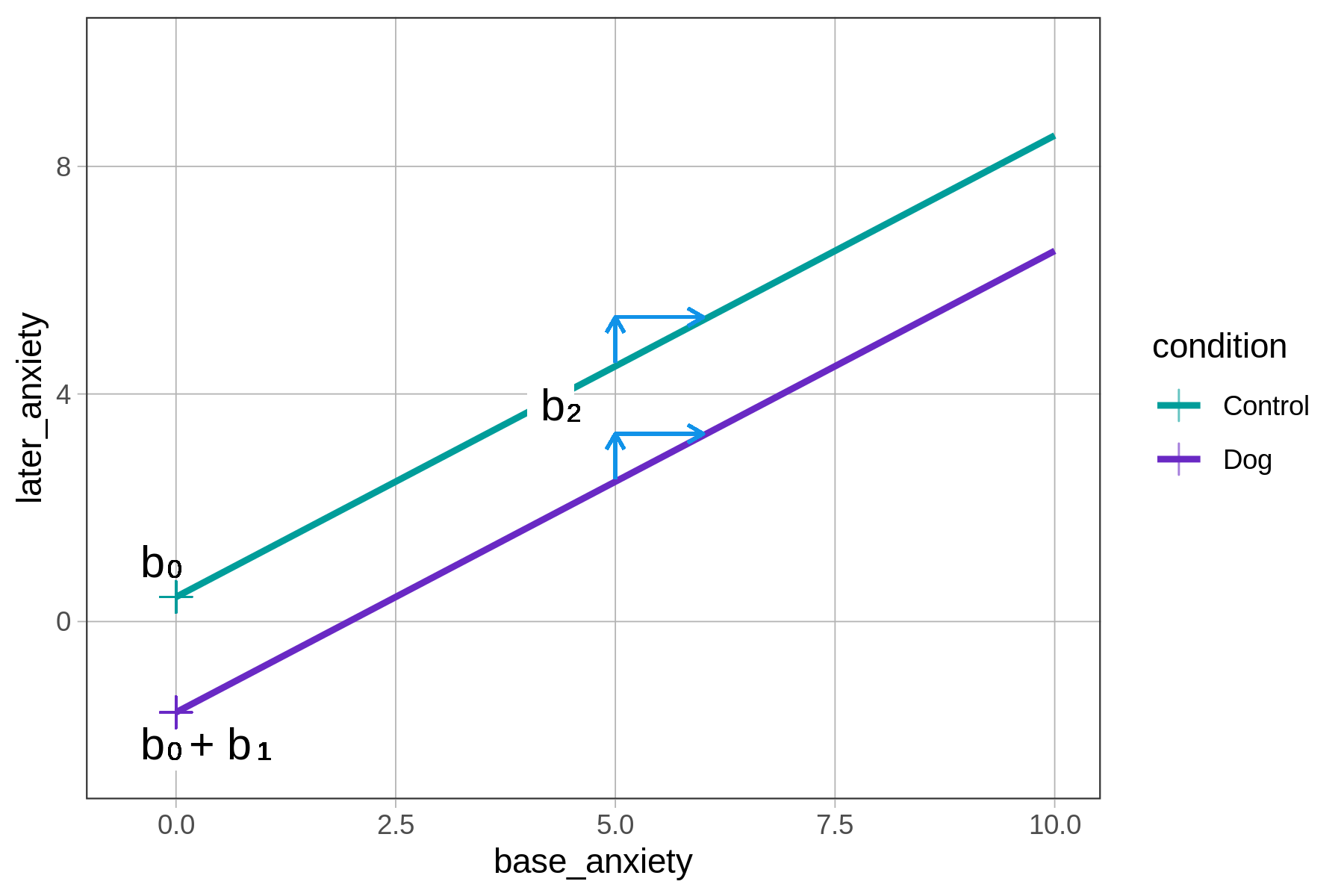
Because the model is additive, the regression lines are constrained to be parallel. For this reason, a single parameter estimate (\(b_2\)) is all that is needed to represent the slope of both lines.
The group difference is represented by the different intercepts of the two parallel lines. For patients in the control group the intercept is \(b_0\). For patients in the dog group the intercept is \(b_0+b_1\). The average difference between the two conditions is \(b_1\), and it is not affected by base anxiety.
\[\text{later}_i = b_0 + \underbrace{b_1\text{Dog}_i}_{\substack{\text{adjustment to} \\ \text{y-intercept} \\ \text{when Dog}_i = 1 }} + b_2\text{base}_i\]
Imagining a Non-Additive Model
You now have some sense of what an additive model is. But what is the alternative to an additive model? One alternative is what generally is referred to as an interaction model.
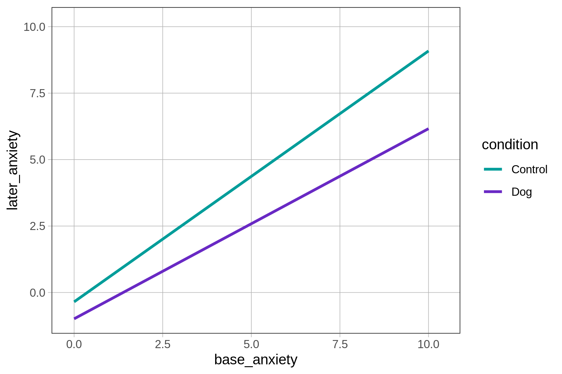
| Additive Model | Interaction Model |
|---|---|
|
|
|
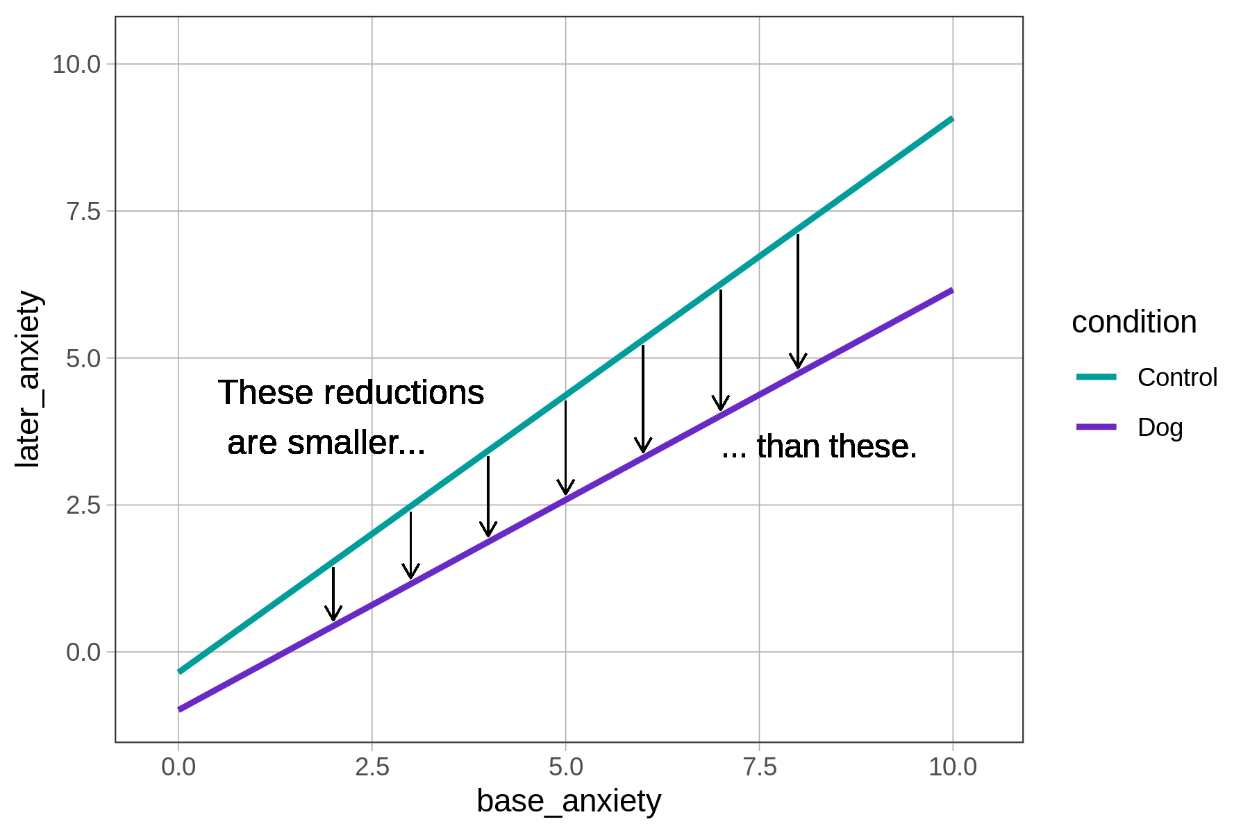
More specifically, the interaction model depicted above predicts that for each unit increase in base anxiety, having a therapy dog assigned will result in a bigger reduction in later anxiety (shown by how the vertical black lines increase in size, left to right).
Definition of an interaction: An interaction model is one in which the relationship of one predictor to the outcome variable depends on the value of a second predictor.
In a model like this one, with one quantitative and one categorical predictor, the interaction of the two predictors will result in two regression lines that are not parallel to each other.
If we choose to go with the interaction model, and if someone asks us, “What’s the relationship between base anxiety and later anxiety?”, we would have to answer like this: “It depends on which condition they were in.” This is the way it works with interactions.