9.6 Centering a Quantitative Predictor at 0
Let’s take this idea of re-centering the quantitative predictor and run with it. We will first create a new version of the predictor that is centered at 0, and then use this centered variable instead of the original variable in our model.
We could use this code to create a new “centered” variable called base_0:
er$base_0 <- er$base_anxiety - mean(er$base_anxiety)
In the window below, we have put in the code to create the new centered variable. Add some code to get the favstats() for both base_anxiety and the new variable, base_0, and take a look at the results.
require(coursekata)
# this codes centers base anxiety at its mean
er$base_0 <- er$base_anxiety - mean(er$base_anxiety)

# write code to generate the favstats for base_anxiety and base_0
# this codes centers base anxiety at its mean
er$base_0 <- er$base_anxiety - mean(er$base_anxiety)

# write code to generate the favstats for base_anxiety and base_0
favstats(~base_anxiety, data=er)
favstats(~base_0, data=er)
ex() %>% {
  check_function(., "favstats", index = 1) %>%
    check_result() %>%
    check_equal()
  check_function(., "favstats", index = 2) %>%
    check_result() %>%
    check_equal()
}Here are the favstats() for the original variable (base_anxiety) and the new transformed version of the variable centered at 0 (base_0). The mean of the new transformed variable (base_0) is 4.229731e-16 which is very close to 0.
       min        Q1     median       Q3      max         mean       sd  n missing
         0         4          6        8       10     6.119048 2.748076 84       0

       min        Q1     median       Q3      max         mean       sd  n missing
 -6.119048 -2.119048 -0.1190476 1.880952 3.880952 4.229731e-16 2.748076 84       0
Re-Fitting the Interaction Model with Base Anxiety Centered at 0
Let’s now re-fit the interaction model with the new centered variable.
Because the meaning of 0 has changed when we substitute base_0 as the predictor, the best-fitting estimate of \(b_1\), which is the effect of being in the dog group when base anxiety is 0, will also change.
In the code window below we’ve included code to fit and print estimates for the original interaction model using condition and base_anxiety as predictors. We’ve also added code to create the centered variable base_0. Add code to fit the same model using base_0 instead of base_anxiety and print out the new estimates.
require(coursekata)
# fits old interaction model and prints estimates
lm(later_anxiety ~ condition * base_anxiety, data = er)

# creates a new variable for base anxiety centered at 0
er$base_0 <- er$base_anxiety - mean(er$base_anxiety)

# write code to fit and print estimates
# for an interaction model substituting base_0 for base_anxiety
lm(later_anxiety ~ condition * base_0, data = er)
ex() %>%
  check_function("lm", index = 2) %>%
  check_result() %>%
check_equal()Let’s compare the model estimates for the interaction model when using condition and base_anxiety as predictors with those obtained when we substitute base_0 for base_anxiety.
The Uncentered Model (with base_anxiety)
Call:
lm(formula = later_anxiety ~ condition * base_anxiety, data = er)

Coefficients:
              (Intercept)               conditionDog
                  -0.3506                    -0.6388
             base_anxiety  conditionDog:base_anxiety
                   0.9437                    -0.2285
The Centered Model (with base_0)
Call:
lm(formula = later_anxiety ~ condition * base_0, data = er)

Coefficients:
              (Intercept)               conditionDog
                   5.4239                    -2.0368
                   base_0        conditionDog:base_0
                   0.9437                    -0.2285
Notice how the \(b_1\) estimate changes when we center base anxiety at 0. Using base_anxiety in the model produces an estimate of -0.64, whereas using base_0 we get an estimate of -2.04. The decrease in anxiety from being in the dog group appears larger using the centered version of base anxiety.
Of course, the overall size of the effect has not changed just because we transformed the variable. Instead, it’s just the meaning of 0 on the base anxiety scale that has changed. Remember, \(b_1\) is the estimated effect of being in the dog group when base anxiety is 0.
In the original model (left panel of the figure below), 0 was the lowest possible level of base anxiety. For patients who started out being this low in anxiety, being in the dog group could not possibly have made their anxiety any lower, which explains why the \(b_1\) estimate is so low.
When we centered base anxiety at 0, however (right panel of the figure), the estimate of \(b_1\) represents the predicted effect of being in the dog group when a patient starts out with an average level of anxiety (the new 0). For these patients, being in the dog group has a larger effect. In general, patients with more than average anxiety are predicted to be more affected by having a therapy dog, patients with less than average anxiety, less affected.
later_anxiety ~ condition * base_anxiety
|
later_anxiety ~ condition * base_0
|
|---|---|
|
|
|
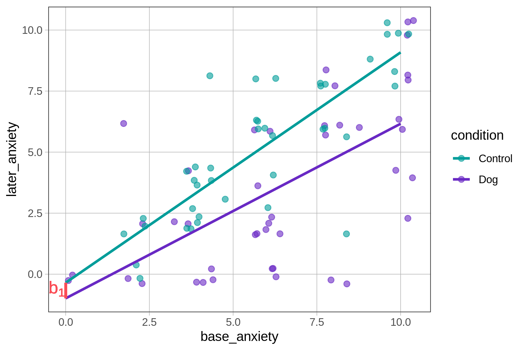
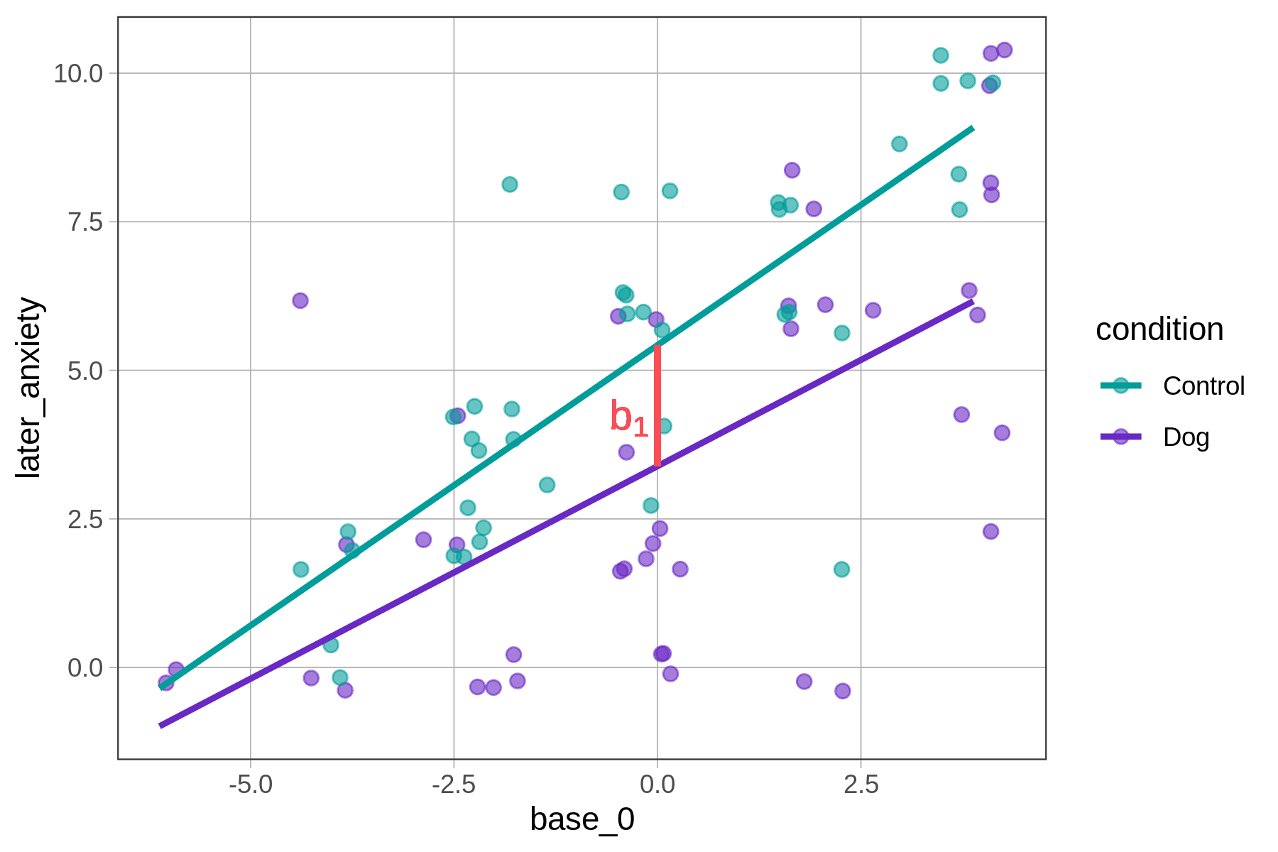
Notice that the slopes of the two lines representing the model predictions do not change just because we centered base anxiety at 0. The slope for the control group is 0.94 (\(b_2\)), and the slope for the dog group is 0.94 + -0.23 (i.e., \(b_2+b_3\)). (You can confirm this visually in the two graphs above as well.)