9.7 Comparing the Interaction Model to the Additive Model (Part 1)
Error from the interaction model is calculated just as it is for the other models we have considered. A model prediction is generated for each patient’s later anxiety based on their values on the predictor variables, and this predicted later_anxiety is then subtracted from the patient’s actual later_anxiety to get a residual.
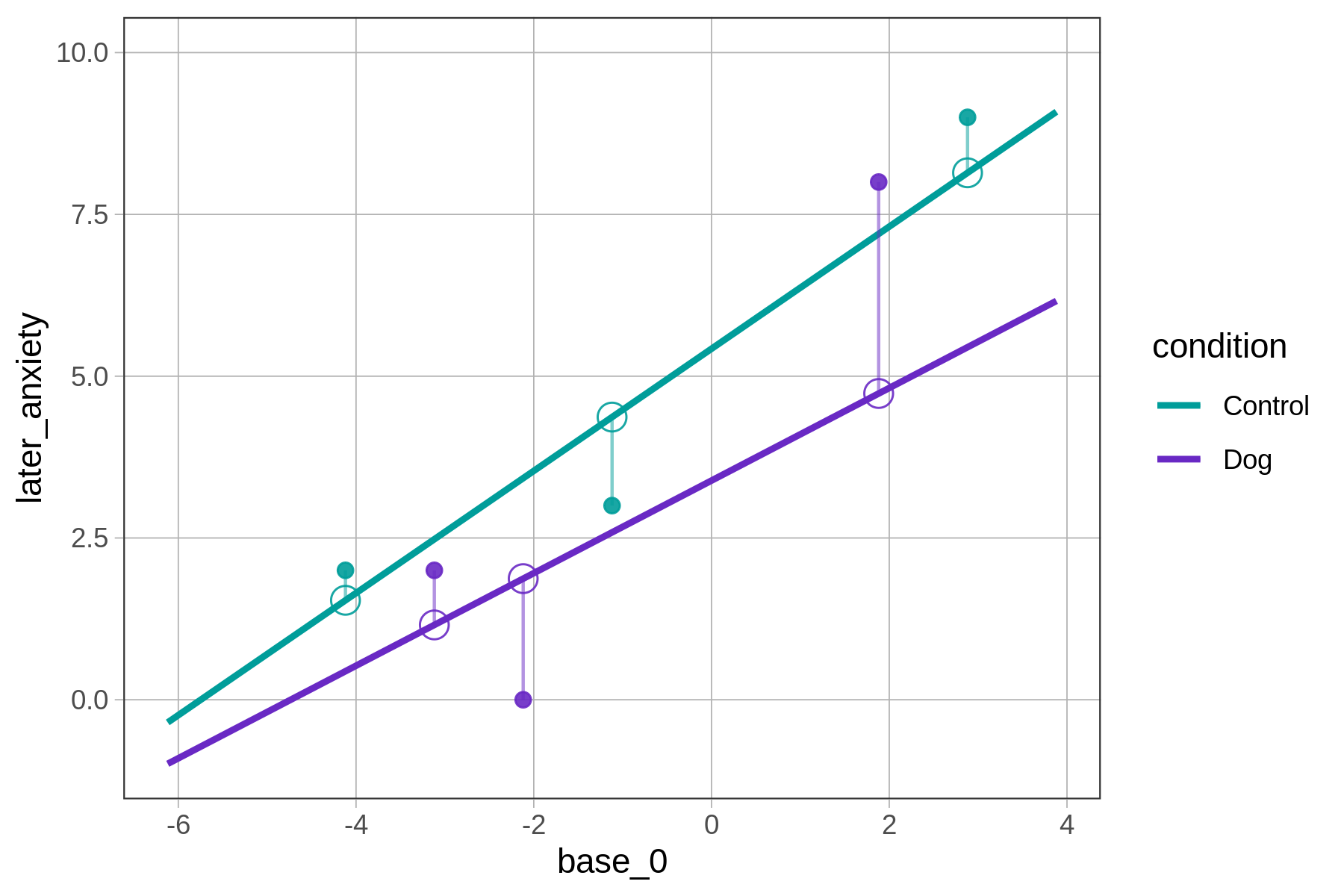
A few of these individual residuals are shown below. The solid dots represent the data for the six patients included in the graph. The empty dots represent the model predictions for each of these patients based on the interaction model. Notice that the model predictions all fall right on the model’s regression lines. The vertical lines represent the residuals for each data point.
These individual residuals are then squared, summed, and used to create Sums of Squares that comprise the foundation of the ANOVA table.
ANOVA Table for the Interaction Model
In the code window below, generate an ANOVA table for the interaction model (we’ve fit and saved the model already).
require(coursekata)
er$base_0 <- er$base_anxiety - mean(er$base_anxiety)
# this saves the best-fitting interaction model
interaction_model <- lm(later_anxiety ~ condition * base_0, data = er)

# generate the ANOVA table
# this saves the best-fitting interaction model
interaction_model <- lm(later_anxiety ~ condition * base_0, data = er)

# generate the ANOVA table
supernova(interaction_model)
ex() %>%
  check_function("supernova") %>%
  check_result() %>%
check_equal()Analysis of Variance Table (Type III SS)
Model: later_anxiety ~ condition * base_0
SS df MS F PRE p
---------------- --------------- | ------- -- ------- ------ ------ -----
Model (error reduced) | 477.433 3 159.144 34.991 0.5675 .0000
condition | 86.527 1 86.527 19.025 0.1921 .0000
base_0 | 232.976 1 232.976 51.224 0.3904 .0000
condition:base_0 | 7.922 1 7.922 1.742 0.0213 .1907
Error (from model) | 363.853 80 4.548
---------------- --------------- | ------- -- ------- ------ ------ -----
Total (empty model) | 841.286 83 10.136 Interpretation of this table is, in most respects, similar to that of the ANOVA table that we have seen from other models (additive models and one-predictor models). But there are some important differences.
The most important rows in this table are the first one (Model) and the fourth one, for the interaction term (condition:base_0). Let’s consider them one at a time.
The Model Row
The interpretation of the first row is the same as it is in all the models we have looked at. It summarizes the comparison of the overall model (in this case the interaction model) with the empty model.
Analysis of Variance Table (Type III SS)
Model: later_anxiety ~ condition * base_0

                                         SS df      MS      F    PRE     p
 ---------------- --------------- | ------- -- ------- ------ ------ -----
            Model (error reduced) | 477.433  3 159.144 34.991 0.5675 .0000
        condition                 |  86.527  1  86.527 19.025 0.1921 .0000
           base_0                 | 232.976  1 232.976 51.224 0.3904 .0000
 condition:base_0                 |   7.922  1   7.922  1.742 0.0213 .1907
            Error (from model)    | 363.853 80   4.548
 ---------------- --------------- | ------- -- ------- ------ ------ -----
Total (empty model) | 841.286 83 10.136 The Model Row for the Interaction vs. Additive Models
It is useful to compare the Model row of the interaction model to the additive model we fit previously. The PRE for the interaction model is .57, whereas for the additive model it is .56 (see the two ANOVA tables, below).
Interaction Model
Analysis of Variance Table (Type III SS)
 Model: later_anxiety ~ condition + base_0 + condition * base_0

                         SS df      MS      F    PRE     p
 ---------------- | ------- -- ------- ------ ------ -----
 Model            | 477.433  3 159.144 34.991  0.5675 .0000
 condition        |  86.527  1  86.527 19.025 0.1921 .0000
 base_0           | 232.976  1 232.976 51.224 0.3904 .0000
 condition:base_0 |   7.922  1   7.922  1.742 0.0213 .1907
 Error            | 363.853 80   4.548
 ---------------- | ------- -- ------- ------ ------ -----
 Total            | 841.286 83  10.136
Additive Model
Analysis of Variance Table (Type III SS)
 Model: later_anxiety ~ condition + base_0

                  SS df      MS      F    PRE     p
 --------- | ------- -- ------- ------ ------ -----
 Model     | 469.512  2 234.756 51.147  0.5581 .0000
 condition |  85.790  1  85.790 18.691 0.1875 .0000
 base_0    | 409.948  1 409.948 89.317 0.5244 .0000
 Error     | 371.774 81   4.590
 --------- | ------- -- ------- ------ ------ -----
 Total     | 841.286 83  10.136
Given that we used an additional degree of freedom to fit the interaction model (3 versus the additive model’s 2), we might very well question, just based on these PREs, whether the interaction model is worth it. All we gained by letting the slopes differ within the two conditions was an additional .01 of PRE.
Although the PRE for the interaction model is larger than for the additive model, the F statistic is considerably smaller (35 versus 51). This is because the F statistic helps us to balance the additional PRE gained with the simplicity we are giving up by adopting the interaction model.