12.2 What You have Learned about Modeling Variation
At first, this was all we could do. You could spot a relationship in a graph, but you weren’t able to quantify it. But now you can do so much more! You can actually specify and fit models to the data, and figure out how strong the relationship is!
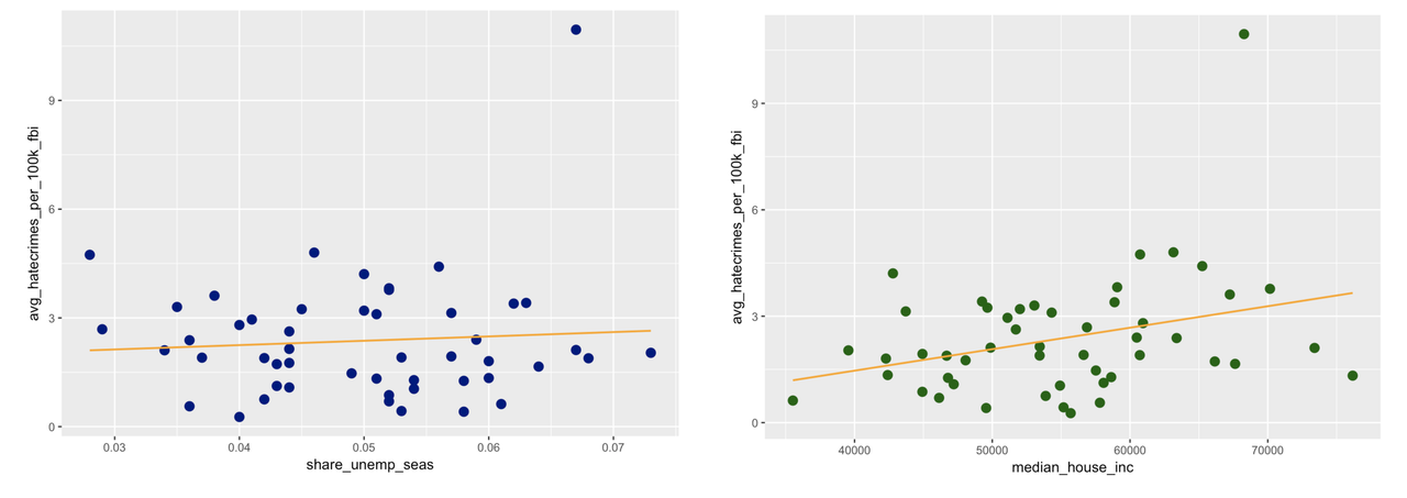
Below we’ve re-drawn the graphs to include the best-fitting regression line. (You totally could have done this yourself; feel free to go back and try it if you want.)
Use the code window below to find the best-fitting estimates of these two models.
require(coursekata)
# find and print the best-fitting estimates for the unemployment model


# find and print the best-fitting estimates for the income model
# find and print the best-fitting estimates for the unemployment model
lm(avg_hatecrimes_per_100k_fbi ~ share_unemp_seas, data = hate_crimes)

# find and print the best-fitting estimates for the income model
lm(avg_hatecrimes_per_100k_fbi ~ median_house_inc, data = hate_crimes)
not_called = "Did you use the lm() function to find and print the best-fitting estimates?"
ex() %>% {
    check_function(., "lm", index = 1, not_called_msg = not_called) %>% check_result() %>% check_equal(incorrect_msg = "Did you model avg_hatecrimes_per_100k_fbi as a function of share_unemp_seas in the hate_crimes data frame?")

    check_function(., "lm", index = 2, not_called_msg = not_called) %>% check_result() %>% check_equal(incorrect_msg = "Did you model avg_hatecrimes_per_100k_fbi as a function of median_house_inc in the hate_crimes data frame?" )
}Call:
lm(formula = avg_hatecrimes_per_100k_fbi ~ share_unemp_seas, data = hate_crimes)
Coefficients:
(Intercept) share_unemp_seas
1.77 11.99
Call:
lm(formula = avg_hatecrimes_per_100k_fbi ~ median_house_inc, data = hate_crimes)

Coefficients:
     (Intercept)  median_house_inc
      -9.564e-01         6.054e-05
Just from our visualizations, we got the impression that the median household income would explain more of the variation in hate crimes than would unemployment. But median household income has a very small slope: .00006, compared to 11.99 for unemployment.
You know by now that to get these statistics, you will need to examine the ANOVA tables for the two models. How did you ever get along without the supernova() function before? Use the code window below (where we have fit two models for you: unemp.model and income.model) to get the ANOVA tables for the two models.
require(coursekata)
# this code fits the models
unemp.model <- lm(avg_hatecrimes_per_100k_fbi ~ share_unemp_seas, data = hate_crimes)
income.model <- lm(avg_hatecrimes_per_100k_fbi ~ median_house_inc, data = hate_crimes)

# print the supernova table for unemp.model


# print the supernova table for income.model
# this code fits the models
unemp.model <- lm(avg_hatecrimes_per_100k_fbi ~ share_unemp_seas, data = hate_crimes)
income.model <- lm(avg_hatecrimes_per_100k_fbi ~ median_house_inc, data = hate_crimes)

# print the supernova table for unemp.model
supernova(unemp.model)

# print the supernova table for income.model
supernova(income.model)
msg = "Did you call supernova() on both unemp.model and income.model?"
ex() %>% {
    check_output_expr(., "supernova(unemp.model)")
    check_output_expr(., "supernova(income.model)")
}Analysis of Variance Table (Type III SS)
Model: avg_hatecrimes_per_100k_fbi ~ share_unemp_seas
SS df MS F PRE p
----- --------------- | ------- -- ----- ----- ------ -----
Model (error reduced) | 0.787 1 0.787 0.264 0.0055 .6099
Error (from model) | 143.206 48 2.983
----- --------------- | ------- -- ----- ----- ------ -----
Total (empty model) | 143.993 49 2.939 Analysis of Variance Table (Type III SS)
Model: avg_hatecrimes_per_100k_fbi ~ median_house_inc
SS df MS F PRE p
----- --------------- | ------- -- ------ ----- ------ -----
Model (error reduced) | 14.584 1 14.584 5.409 0.1013 .0243
Error (from model) | 129.409 48 2.696
----- --------------- | ------- -- ------ ----- ------ -----
Total (empty model) | 143.993 49 2.939 From the two models we fit here, we would say that the income model explains more variation in hate crimes than does the unemployment model. States with higher household incomes seem to report more hate crimes to the FBI. This relationship isn’t perfectly predictive, but it does explain 10% of the total error around the empty model.