Chapter 5 - A Simple Model

5.1 A Simple Model

In this section we will start with the concept of model, and then develop the concept of statistical model. We present a simple model, the empty model, and from there begin developing the important concept of error. We also will introduce some mathematical notation for describing statistical models.

What Is a Model, and Why Would We Want One?

You may have heard people talk about statistical models. Someone may say, “I built a model based on the data,” or, “Our model predicts that… .” Most people who hear such statements just nod their heads, knowingly. But inside they are wondering: what does that mean?

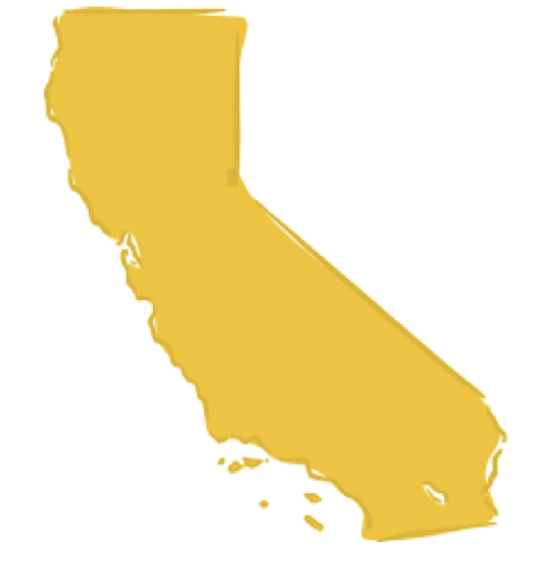
We introduce the idea of a model by analogy. Let’s say you want to estimate the area in square miles of the the State of California. (Assume, for the moment, that you can’t just look it up in Wikipedia!) This is not easy, because California is a large and irregularly shaped state, as pictured below.

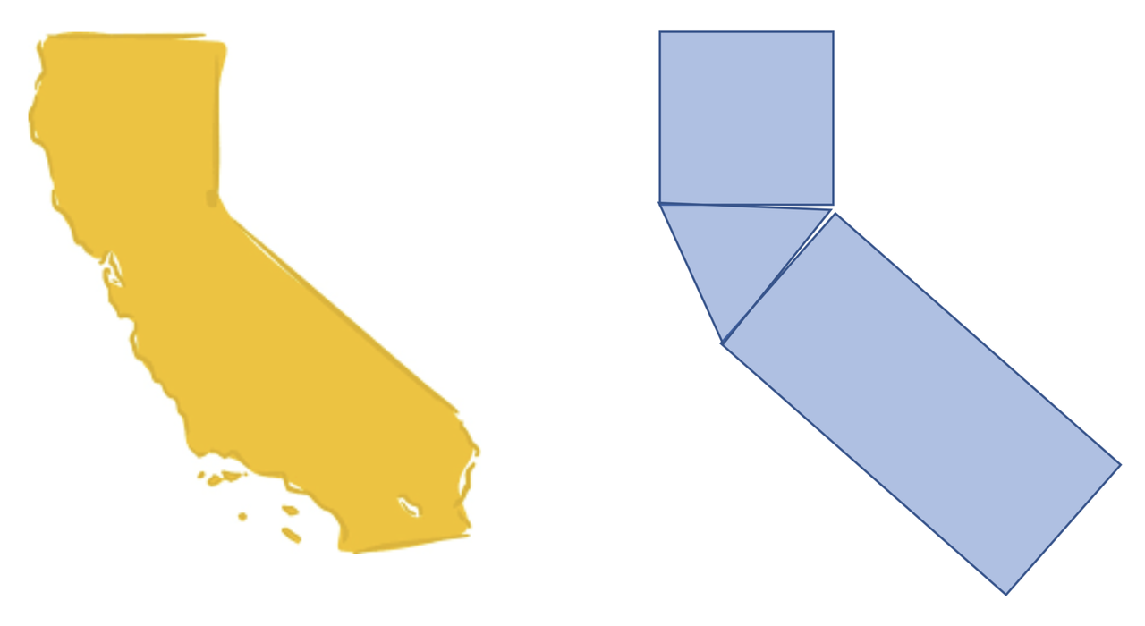
One way to go about this would be to model the area of the state using geometric figures—specifically, rectangles and triangles. If we draw two rectangles and a triangle, and put them together in the right way, we can get something that looks somewhat like California.

One thing to notice about our model at the outset is that it is not very good. Most models, in fact, are pretty bad. Although the model is vaguely California-like, there are a lot of details that are not captured in the model. But, it is better than nothing! And, because we know how to calculate the area of a rectangle and the area of a triangle, if we are willing to assume the model is good enough, we can easily calculate an estimate for the area of the state.

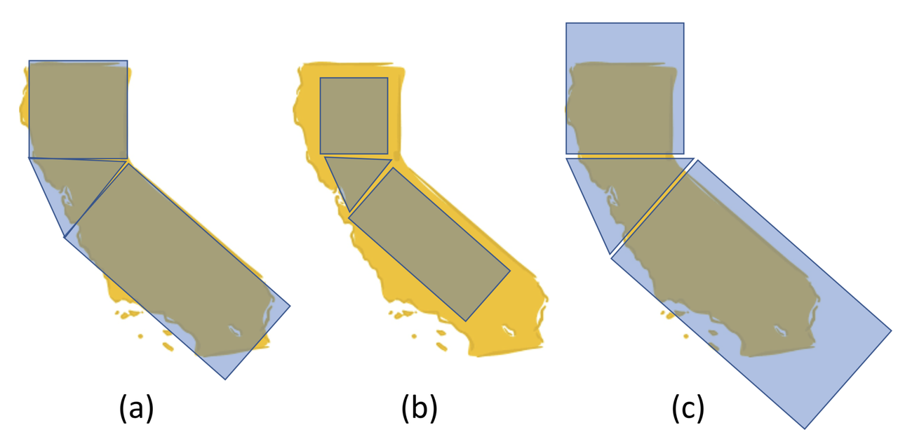
Let’s take the analogy a little further. Once we have decided to model the area of California as two rectangles and a triangle, we try to make the model fit as well as possible. To do this we adjust the size and placement of the geometric shapes. Here are a few examples:

Notice that in panel c, our model seems like it will overestimate the area of California, because we’ve made the shapes too big. In panel b, the model looks like it will result in an underestimate. The model in panel a, however, looks pretty good. We might say that the model in panel a is the “best-fitting model” of the three.

Note that our judgment of fit comes from looking at both the area within the state that is not covered by our model (see the yellow parts sticking out in panel b), and the area not in the state that is covered by the model (see blue parts that are not overlapping with California in panel c). It is useful to think of these two areas as deviations from the model, or error.

If we write a word equation to represent this model, it might look something like this:

AREA OF CALIFORNIA = AREA OF GEOMETRIC FIGURES + OTHER STUFF

The “other stuff” would be the deviations, both positive and negative, from the model. It is useful to think of the best fitting model as the one that minimizes the deviations (or error), making the “other stuff” as small as possible.

Now that we have models, we can be more specific about what we mean by “other stuff.” The “other stuff” becomes error from the model and we can rewrite our word equation like this:

AREA OF CALIFORNIA = AREA OF GEOMETRIC FIGURES + ERROR

Finally, it is also important to note that our geometric model of California is a gross oversimplification of all the different attributes of California one might be interested in. Models are always like this: they oversimplify some aspects of the world, and focus in on only that dimension you are most interested in.