6.4 Standard Deviation
The standard deviation (written as \(s\)) is simply the square root of the variance. We generally prefer thinking about error in terms of standard deviation because it yields a number that makes sense using the original scale of measurement. So, for example, if you were modeling weight in pounds, variance would express the error in square pounds (not something we are used to thinking about), whereas standard deviation would express the error in pounds.
Here are two equivalent formulas that represent the standard deviation.
\[s = \sqrt{s^2}\]
\[\sqrt{\frac{\sum_{i=1}^n (Y_i-\bar{Y})^2}{n-1}}\]
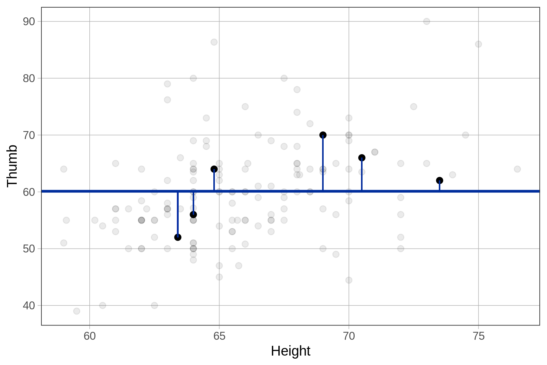
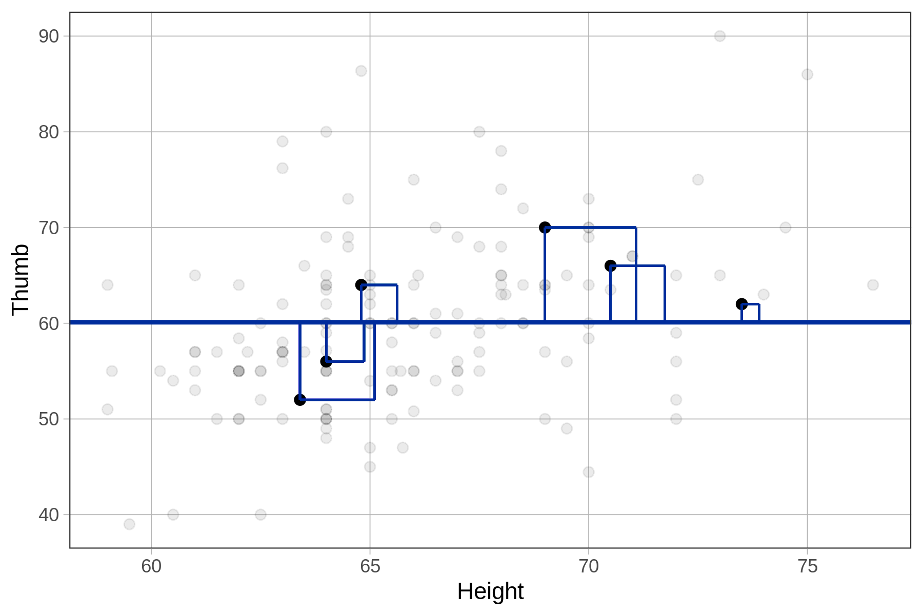
| A few residuals from the empty model | A few squared residuals from the empty model |
|---|---|
|
|
|
To calculate standard deviation in R, we can use the sd() function.
sd(Fingers$Thumb)As with most things in R, there are a variety of ways you could get the standard deviation of a variable other than using the sd() function. You could use a combination of the var() function and the sqrt() function to get the square root of the variance; or you could use favstats(), which includes the standard deviation in its output.
Try all three of these methods in the code window below to calculate the standard deviation of Thumb in the Fingers data frame.
require(coursekata)
empty_model <- lm(Thumb ~ NULL, data = Fingers)
# calculate the standard deviation of Thumb from Fingers with sd()

# calculate the standard deviation with sqrt() and var()

# calculate the standard deviation with favstats()
sd(Fingers$Thumb)
sqrt(var(Fingers$Thumb))
favstats(~Thumb, data = Fingers)
ex() %>% {
    check_function(., "sd") %>% check_result() %>% check_equal()
    check_function(., "sqrt") %>% check_result() %>% check_equal()
    check_function(., "favstats") %>% check_result() %>% check_equal()
}8.726694574660678.72669457466067min Q1 median Q3 max mean sd n missing
39 55 60 65 90 60.10366 8.726695 157 0Sum of Squares, Variance, and Standard Deviation
We have discussed three ways of quantifying error around a model. All start with residuals, but they aggregate those residuals in different ways to summarize total error.
All of them are minimized at the mean, and so all are useful when the mean is the model for a quantitative variable.
Thinking About Quantifying Error in MindsetMatters
Below is a histogram of the amount of weight lost (PoundsLost) by each of the 75 housekeepers in the MindsetMatters data frame.
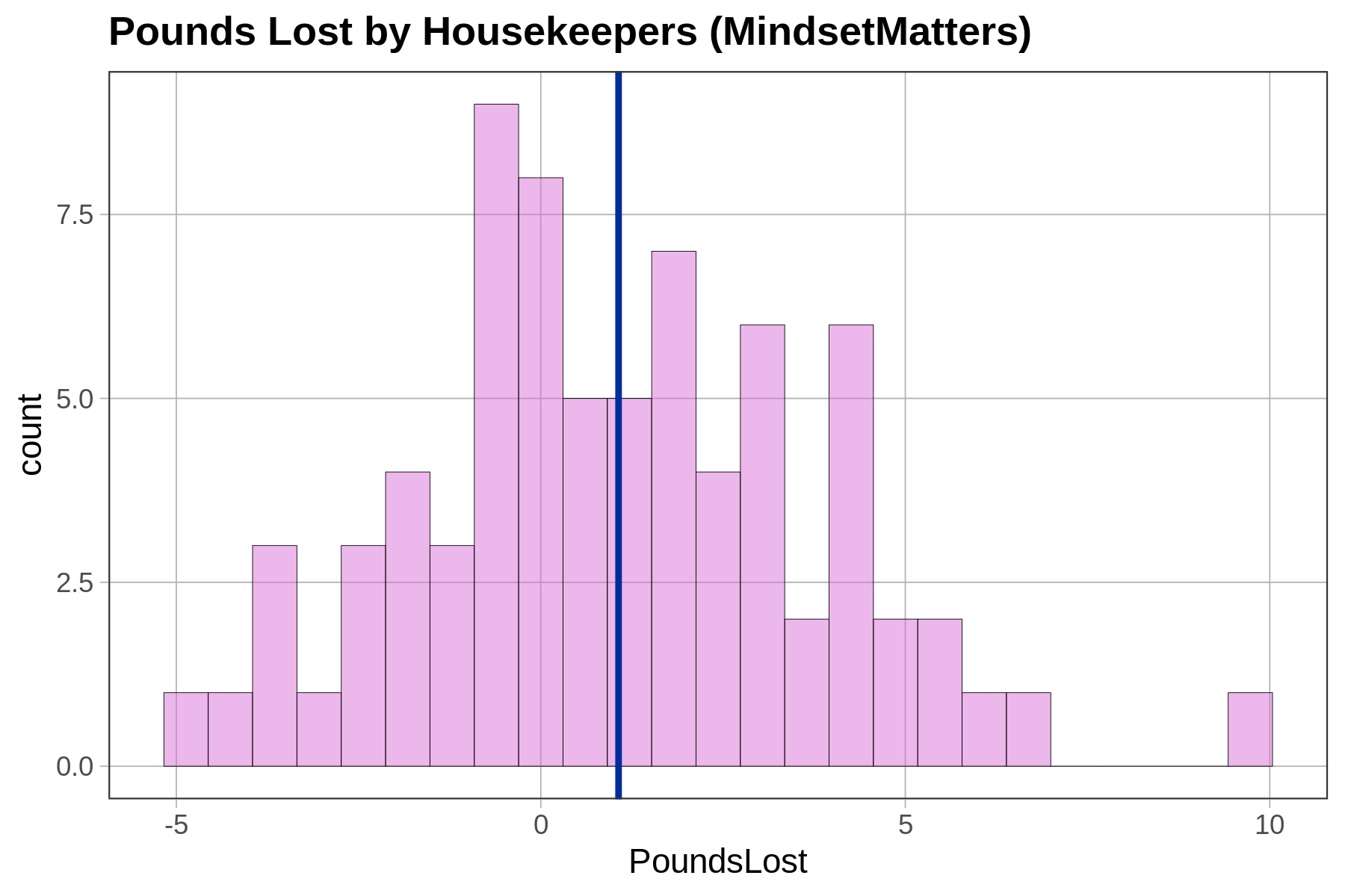
Use R to create an empty model of PoundsLost. Call it empty_model. Then find the SS, variance, and standard deviation of this model.
require(coursekata)
MindsetMatters$PoundsLost <- MindsetMatters$Wt - MindsetMatters$Wt2
# create an empty model of PoundsLost from MindsetMatters
empty_model <-

# find SS, var, and sd
# there are multiple correct solutions
empty_model <- lm(PoundsLost ~ NULL, data = MindsetMatters)
sum(resid(empty_model)^2)
var(MindsetMatters$PoundsLost)
sd(MindsetMatters$PoundsLost)
ex() %>% {
    check_object(., "empty_model") %>% check_equal()
    check_output(., 556.7)
    check_output(., 7.52)
    check_output(., 2.74)
}There are multiple ways to compute these in R, but the results will be the same: SS = 556.73, Variance = 7.52, and Standard Deviation = 2.74.
Notation for Mean, Variance, and Standard Deviation
Finally, we use different symbols to represent the variance and standard deviation of a sample, on one hand, and the population (or DGP), on the other. Sample statistics are also called estimates because in the context of statistical modeling they are used as estimates of the DGP parameters. We have summarized these symbols in the table below (pronunciations for symbols are in parentheses).
| Sample (or estimate) | DGP (or population) | |
|---|---|---|
| Mean | \(\bar{Y}\) (y bar) | \(\mu\) (mu) |
| Variance | \(s^2\) (s squared) | \(\sigma^2\) (sigma squared) |
| Standard Deviation | \(s\) (s) | \(\sigma\) (sigma) |