5.4 Exploring the Mean
It’s pretty easy to understand how the median is the middle of a distribution, but in what sense is the mean the middle? One way to think of the mean is as the balancing point of the distribution, the point at which the things above it equal the things below it. But what does it balance? What are “the things” that are equal on both sides of the mean?
You can either watch the video explanation (with Dr. Ji) or read about it in the section below.
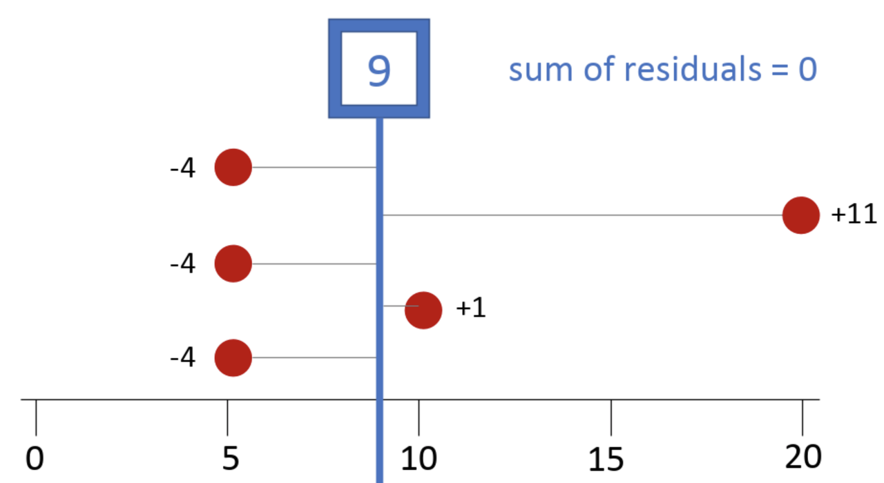
You might think that the values below the mean balance with the values above the mean. Let’s try that. Does 5+5+5 = 10+20? No, 15 does not equal 30. A bunch of smaller values, what we find below the mean, is not going to balance a bunch of larger values (the ones above the mean). So what does the mean balance?
Here it helps to think about each score’s deviation, which is the difference above or below the mean. In our example, each of the 5s are 4 units below the mean of 9, which is a deviation of -4. If you think of it this way, the sum of deviations below the mean (-12) balances out the sum of deviations above the mean (+1 and +11, or +12).
We will also call these differences residuals. The word deviation is specific to differences above and below the mean but residual more generally means differences above and below any model of the distribution, which could be mean, median, mode, etc.
It turns out that no number other than the mean (not 8, not 8.5, not 9.1!) will perfectly balance the residuals above the mean with those below the mean. Whereas the magnitude of a score—especially an outlier—won’t necessarily affect the median, it will affect the mean because the large residual from an outlier has to be balanced with the residuals from the other data points. Every value gets taken into account when calculating the mean.
Remember we talked about finding some simple shapes that “fit” the more detailed shape of California the best? We wanted to find shapes that were not too big and not too small, shapes that would minimize the error around the model, defined as the parts of California that were not covered by the model, and the parts of the model that covered stuff not in California.
The mean is a model that is not too big and not too small. The mean is pulled in both directions (larger and smaller) at once and settles right in the middle. The mean is the number that balances the residuals above and below it, yielding the same amount of error above it as below it. It’s kind of amazing that this procedure of adding up all the numbers and dividing by the number of numbers results in this balancing point.
Thinking about the mean in this way also helps us think about DATA = MODEL + ERROR in a more specific way. If the mean is the model, each data point can now be thought of as the sum of the model (9 in our outcome variable) plus its residual from the model. So 20 can be decomposed into the model part (9) and the error from the model (+11). And 5 can be decomposed into 9 (model) and -4 (error).