7.9 Partitioning Sums of Squares into Model and Error
DATA = MODEL + ERROR
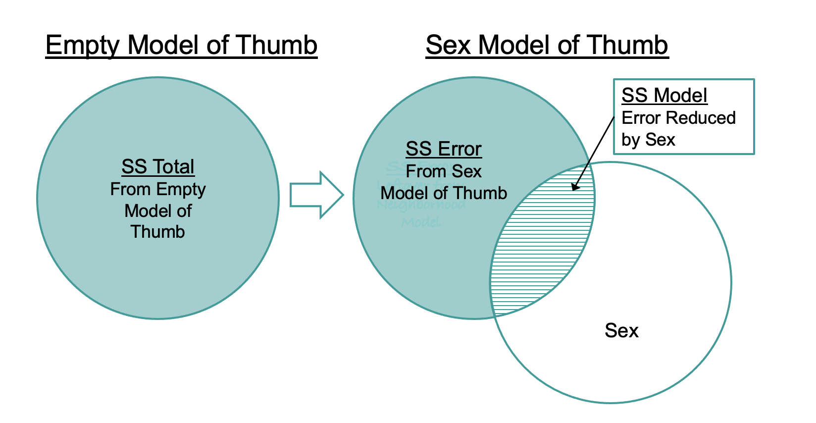
Statistical modeling is all about explaining variation. SS Total tells us how much total variation there is to be explained. When we fit a model (as we have done with the Sex model), that model explains some of the total variation, and leaves some of that variation still unexplained. The part we explain is called SS Model; the part left unexplained, SS Error.
These relationships are visualized in the diagram below: SS Total can be seen as the sum of SS Model (the amount of variation explained by a more complex model) and SS Error, which is the amount left unexplained after fitting the model. Just as DATA = MODEL + ERROR, SS Total = SS Model + SS Error.
Partitioning Sums of Squares
Let’s see how this concept works in the ANOVA table for the sex model (reprinted below). Look just at the column labeled SS (highlighted). The two rows associated with the sex model (Model and Error) add up to the row labeled Total (SS Total for the empty model): 1,334 + 10,546 = 11,880.
Analysis of Variance Table (Type III SS)
Model: Thumb ~ Sex

                               SS  df       MS      F    PRE     p
----- --------------- | --------- --- -------- ------ ------ -----
Model (error reduced) |  1334.203   1 1334.203 19.609 0.1123 .0000
Error (from model)    | 10546.008 155   68.039
----- --------------- | --------- --- -------- ------ ------ -----
Total (empty model)   | 11880.211 156   76.155
Let’s put these numbers back into the Venn diagram of the sex model. SS Total, represented by the whole circle, can be partitioned into two parts: SS Model and SS Error.
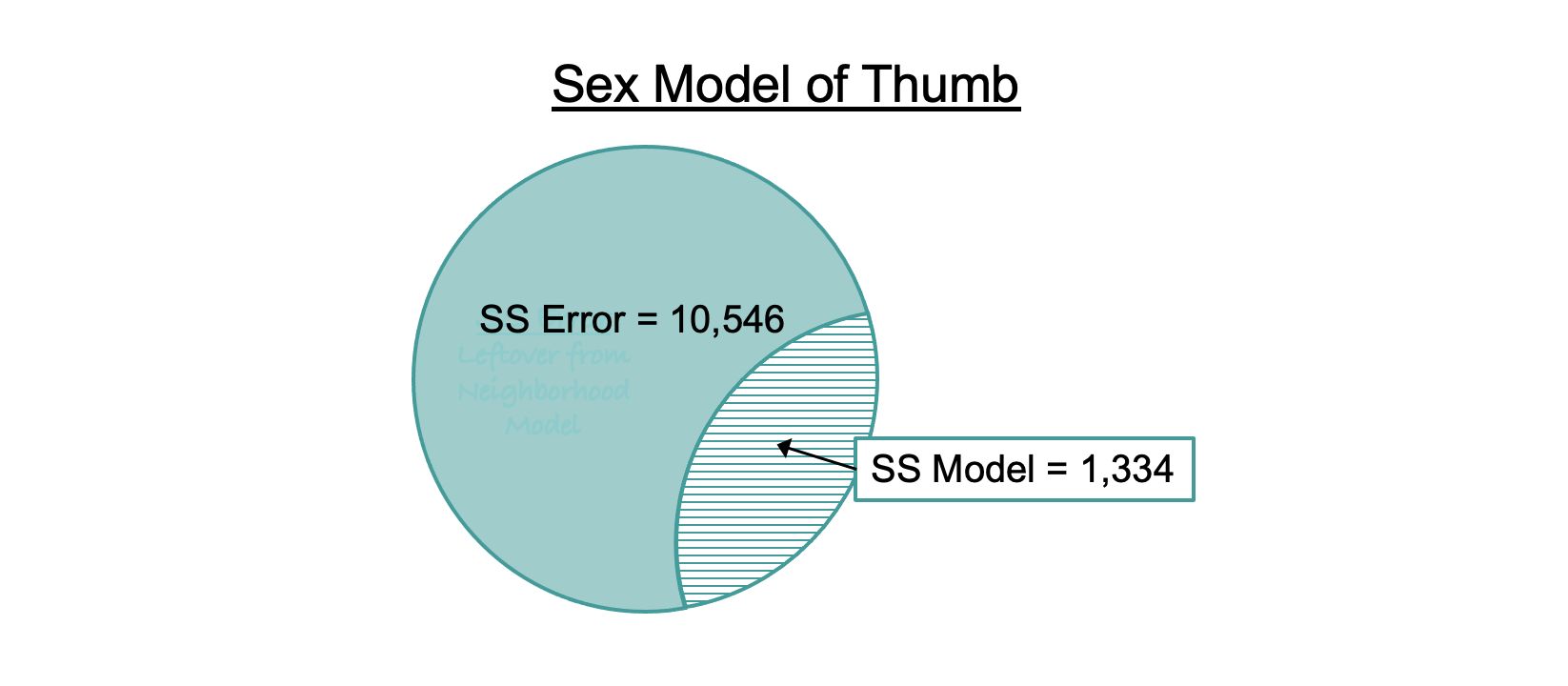
The striped part (SS Model, which is 1,334 for the sex model) represents the part of SS Total that is explained by the sex model. Another way to think of it is as the reduction in error (measured in sums of squares) achieved by the sex model as compared to the empty model.
There are two ways to calculate SS Model. One is to simply subtract SS Error (error from the Sex model predictions) from SS Total (error around the mean, or the empty model):
\[\text{SS}_\text{Model} = \text{SS}_\text{Total} - \text{SS}_\text{Error}\]
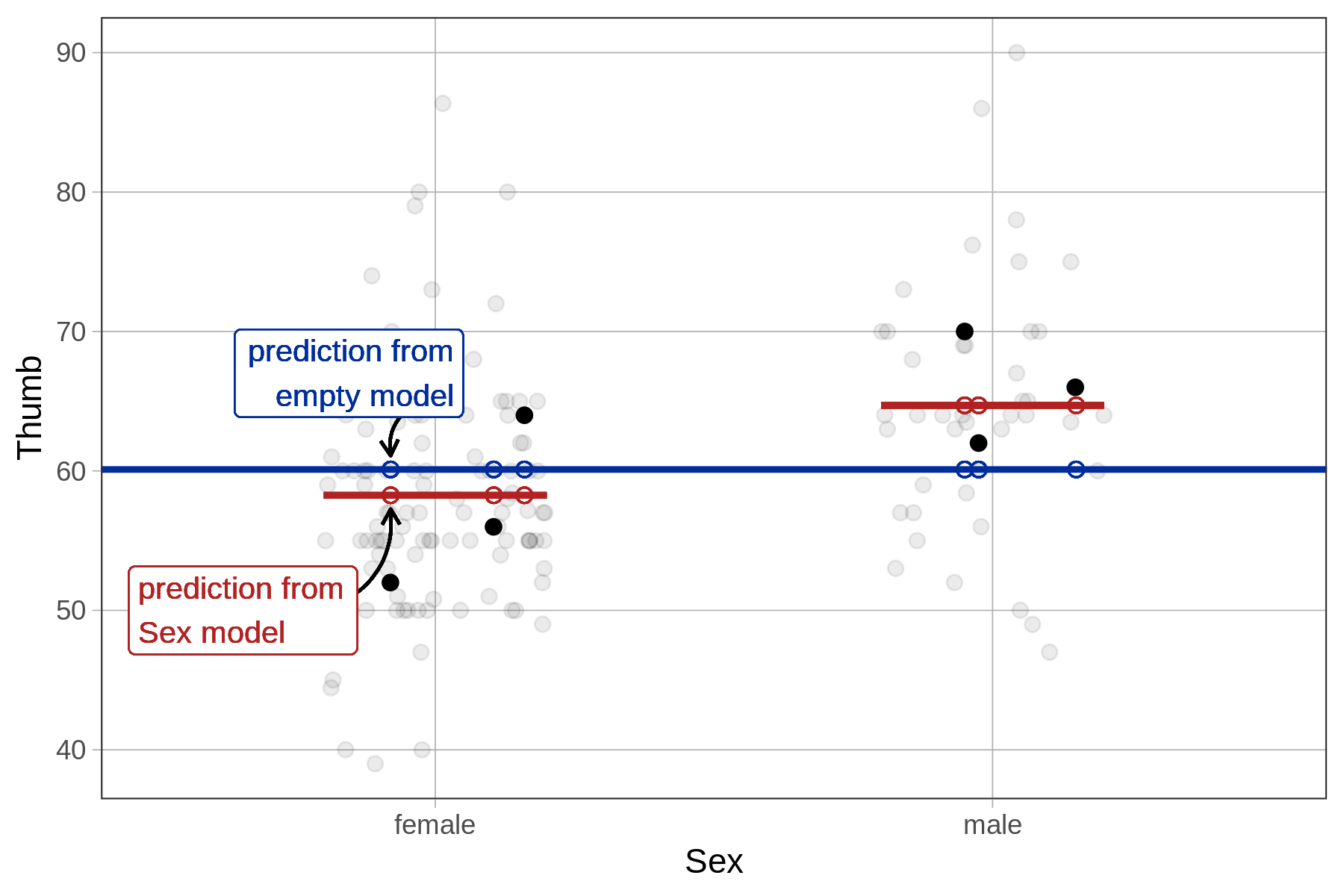
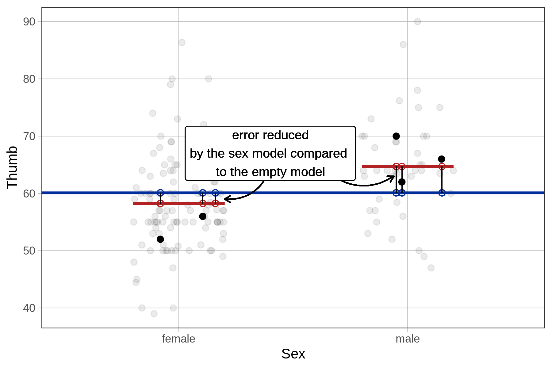
Another way is to calculate the reduction in error from the empty model to the sex model separately for each data point, then square and sum these to get SS Model. As illustrated below for a female student, we take the distance from her predicted score under the sex model to her predicted score under the empty model, then square it. If we do this for each student and then total up the squares we will get SS Model.
The supernova() function tells you that SS Model for the sex model in the Fingers data set is 1,334. But let’s use R to calculate it in this more direct way to see if we get the same result, and further your understanding of what’s going on in the supernova() calculation.
In the code window below, assume the objects empty_model and Sex_model have been created already. The line of code provided generates all the differences between the two model predictions and saves it as a new variable called error_reduced. Run it to see what this variable is like. Then modify that code to square and sum the error reduced to print out SS Model.
require(coursekata)

empty_model <- lm(Thumb ~ NULL, data=Fingers)
Sex_model <- lm(Thumb ~ Sex, data=Fingers)
# creates the differences between the two predictions
error_reduced <-  predict(Sex_model) - predict(empty_model)

# modify this line of code to square and sum these differences
error_reduced
# creates the differences between the two predictions
error_reduced <-  predict(Sex_model) - predict(empty_model)

# modify this line of code to square and sum these differences
sum(error_reduced ^ 2)
ex() %>% check_output(1334.2)1334.20254468864