7.7 Error Reduced by the Group Model
Remember that our goal in adding an explanatory variable to the model was to explain variation in the outcome variable, or to put it another way, reduce error compared with the empty model.
To know that error has been reduced, and by how much it has been reduced, we will compare the sum of squared errors for the empty model with the sum of squared errors from the Sex model. If the sum of squared errors from the Sex model is smaller, then it has reduced error compared to the empty model.
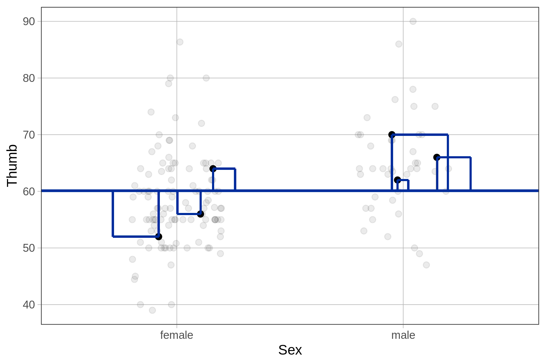
For the empty model, we take each residual from the model prediction (the mean for all students) and square it. Then we add up these squared residuals to get the total sum of squares. The special name we use to refer to the total squared residuals from the empty model is SST, or Sum of Squares Total.
We have illustrated this idea for our subsample of six data points in the left panel of the figure below. The residuals are represented by the vertical lines from each data point to the empty model prediction. The square of each of these residuals is represented, literally, by a square.
| SS Total, Sum of Squared Residuals from empty model |
SS Error, Sum of Squared Residuals from Sex model
|
|---|---|
|
|
|
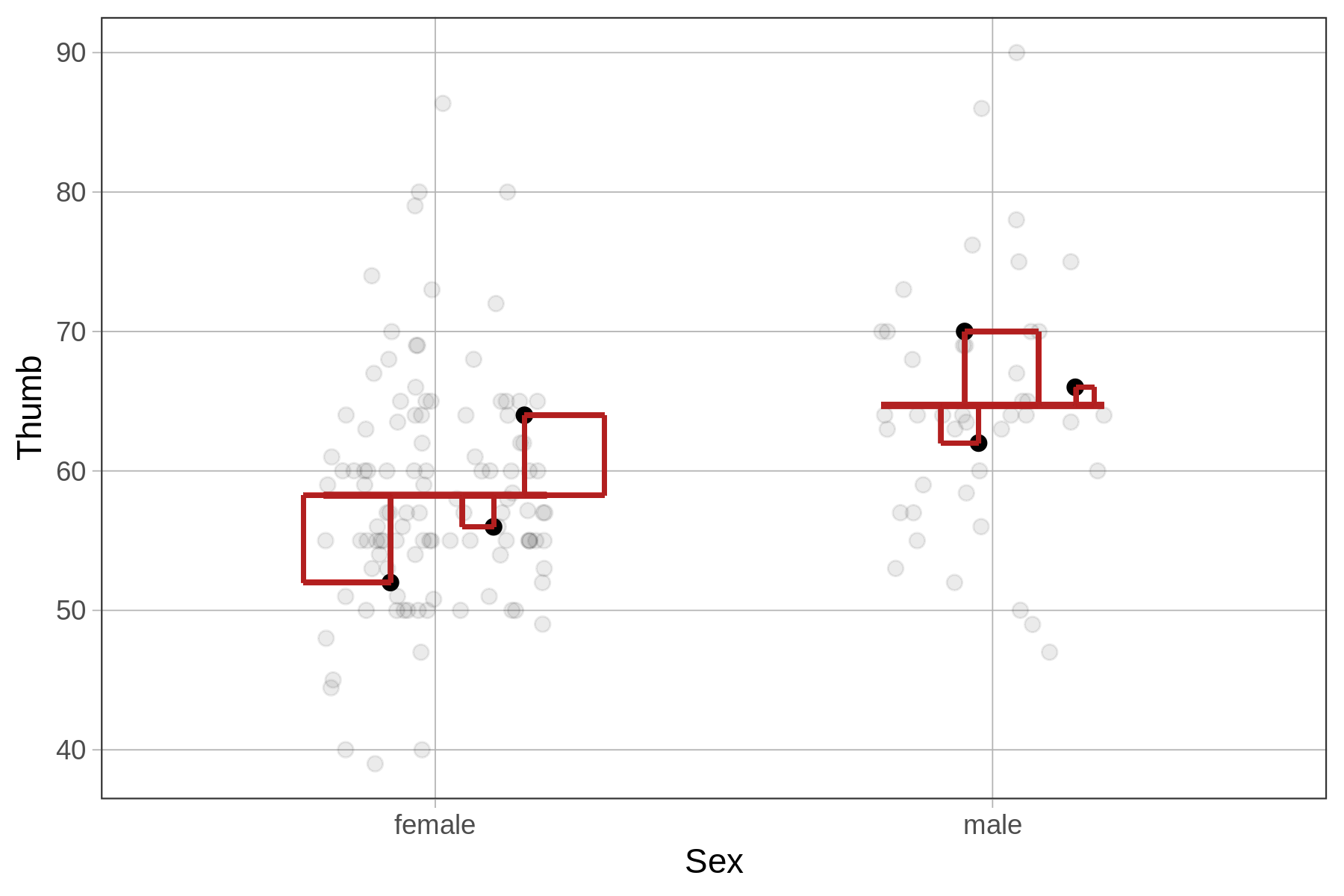
For the Sex model (represented in the right panel of the figure above), we take the same approach, only this time the residuals are based on the model predictions of the Sex model. Again, we can sum up these squared residuals across the whole data set to get the sum of squared errors from the model.
Although the procedure for calculating sums of squares is identical for the empty and Sex models, for the Sex model (and indeed, for all models other than the empty model) we call this sum the SSE, or Sum of Squared Errors.
When R fits a model, the particular values of the parameter estimates (the \(b\)s) minimize the sum of squared residuals.
To fit the empty model, R finds the particular value of \(b_0\) that produces the lowest possible SS Total for this data set, which we know is the mean of Thumb. To fit the Sex model, R finds the particular values of \(b_0\) and \(b_1\) that produce the lowest possible SS Error for this data set.