5.3 The Median vs. Mean as a Model
Having developed the idea that a single number can serve as a statistical model for a distribution, we now ask: which single number should we choose? We have been talking informally about choosing a number in the middle of a symmetric, normal-shaped distribution. But now we want to get more specific.
Recall that in the previous section we defined a statistical model as a function that produces a predicted score for each observation. Armed with this definition, we can now ask: what function could we use that would generate the same predicted value for all observations in a distribution?
Median and Mean: Two Possible Functions for Generating Model Predictions
If we were trying to pick a number to model the distribution of a categorical variable, we should pick the mode; really, there isn’t much choice here. If you are going to predict the value of a new observation on a categorical variable, the prediction will have to be one of the categories and you will be wrong least often if you pick the most frequently observed category.
For a quantitative variable, statisticians typically choose one of two numbers: the median or the mean. The median is just the middle number of a distribution. Take the following distribution of five numbers:
5, 5, 5, 10, 20
The median is 5, meaning that if you sort all the numbers in order, the number in the middle is 5. You can see that the median is not affected by outliers. So, if you changed the 20 in this distribution to 20,000, the median would still be 5.
To calculate the mean of this distribution, we simply add up all the numbers in the sample, and then divide by the sample size, which is 5. So, the mean of this distribution is 9. Both mean and median are indicators of where the middle of the distribution is, but they define “middle” in different ways: 5 and 9 represent very different points in this distribution.
In R, these and other statistics are very easy to find with the function favstats(). Create a variable called outcome and put in these numbers: 5, 5, 5, 10, 20. Then, run the favstats() function on the variable outcome.
require(coursekata)
# Modify this line to save the numbers to outcome
outcome <- c()

# This will give you the favstats for outcome
favstats(outcome)
outcome <- c(5, 5, 5, 10, 20)
favstats(outcome)
ex() %>% {
    check_object(., "outcome") %>% check_equal()
    check_function(., "favstats") %>% check_result() %>% check_equal()
} min Q1 median Q3 max mean sd n missing
5 5 5 10 20 9 6.519202 5 0If our goal is just to find the single number that best characterizes a distribution, sometimes the median is better, and sometimes the mean is better.
If you are trying to choose one number that would best predict what the next randomly sampled value might be, the median might well be better than the mean for this distribution. With only five numbers, the fact that three of them are 5 leads us to believe that the next one might be 5 as well.
On the other hand, we know nothing about the Data Generating Process (DGP) for these numbers. The fact that there are only five of them indicates that this distribution is probably not a good representation of the underlying population distribution. The population could be normal, or uniform, in which case the mean would be a better model than the median. The point is, we just don’t know.
Realizing this limitation, let’s look below at the distributions of several quantitative variables. For each variable, make a histogram and get the favstats(). Then decide which number you think would be a better model for the distribution – the median or the mean.
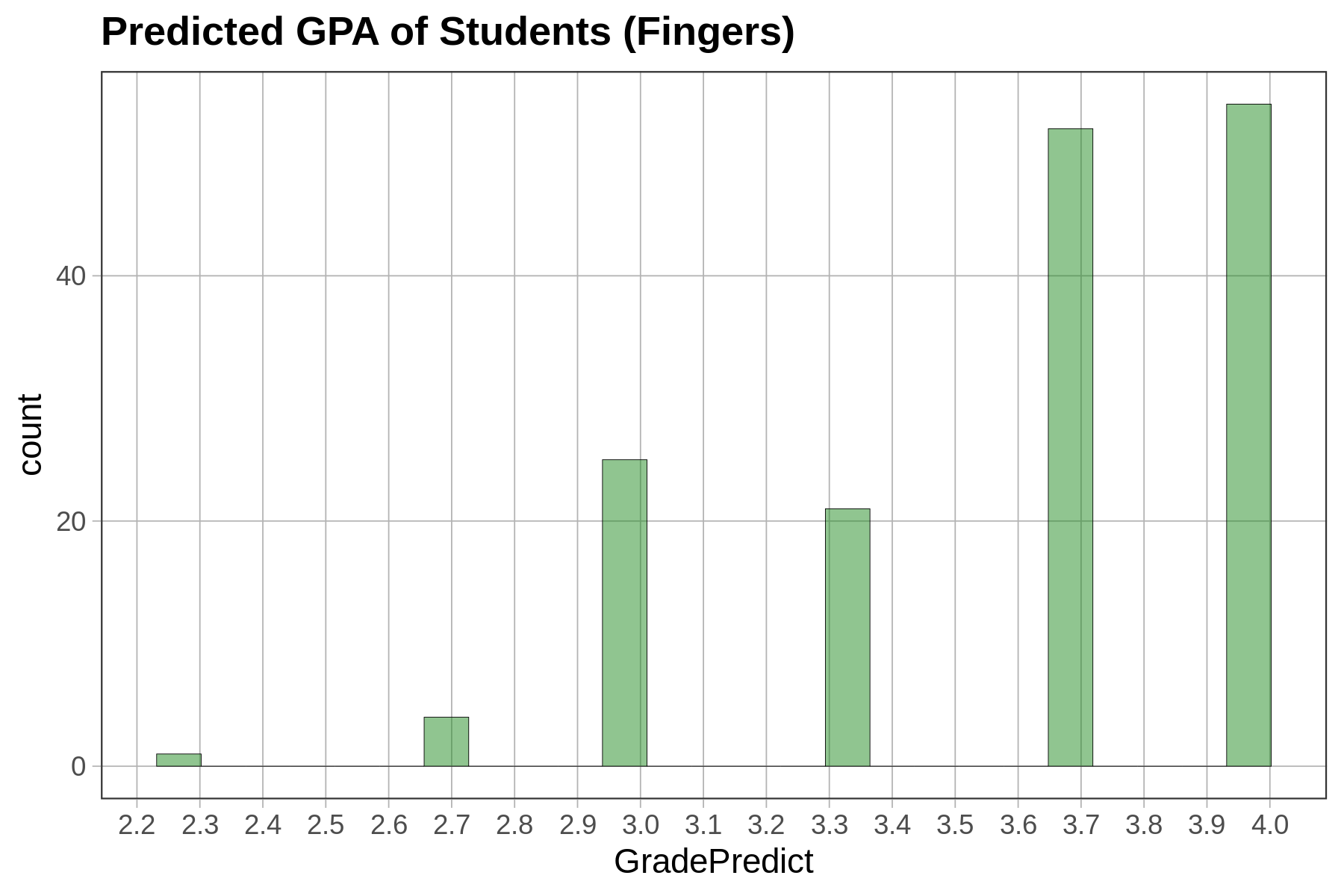
Variable 1: Students’ Self-Predictions of GPA in the Fingers Data Frame
require(coursekata)
# modify this code to make a histogram of GradePredict
# the second line adds more tick marks to the x-axis
gf_histogram(~ , data = Fingers, color = "forestgreen") +
 scale_x_continuous(breaks = seq(2.0, 4.0, by = 0.1))

# modify this code to get the favstats for GradePredict
favstats(~ GradePredict, data = )
# modify this code to make a histogram of GradePredict
# the second line adds more tick marks to the x-axis
gf_histogram(~ GradePredict, data = Fingers, color = "forestgreen") +
 scale_x_continuous(breaks = seq(2.0, 4.0, by = 0.1))

# modify this code to get the favstats for GradePredict
favstats(~ GradePredict, data = Fingers)
ex() %>% {
  check_or(.,
    check_function(., "gf_histogram") %>% {
      check_arg(., "object") %>% check_equal()
      check_arg(., "data") %>% check_equal()
    },
    override_solution(., "gf_histogram(Fingers, ~ GradePredict)") %>%
      check_function("gf_histogram") %>% {
        check_arg(., "object") %>% check_equal()
        check_arg(., "gformula") %>% check_equal()
      },
    override_solution(., "gf_histogram(~ Fingers$GradePredict)") %>%
      check_function("gf_histogram") %>%
      check_arg(., "object") %>%
      check_equal()
  )
  check_function(., "favstats") %>%
    check_result() %>%
    check_equal()
}Note that there are two ways of asking favstats() or gf_histogram() to retrieve a variable that is inside a data frame: by using the $ like this: favstats(Fingers$GradePredict); or by using a combination of ~ and data = like this: favstats(~ GradePredict, data = Fingers). We prefer to use the latter version with the tilde (~) because it will work better with other functions we will learn about.
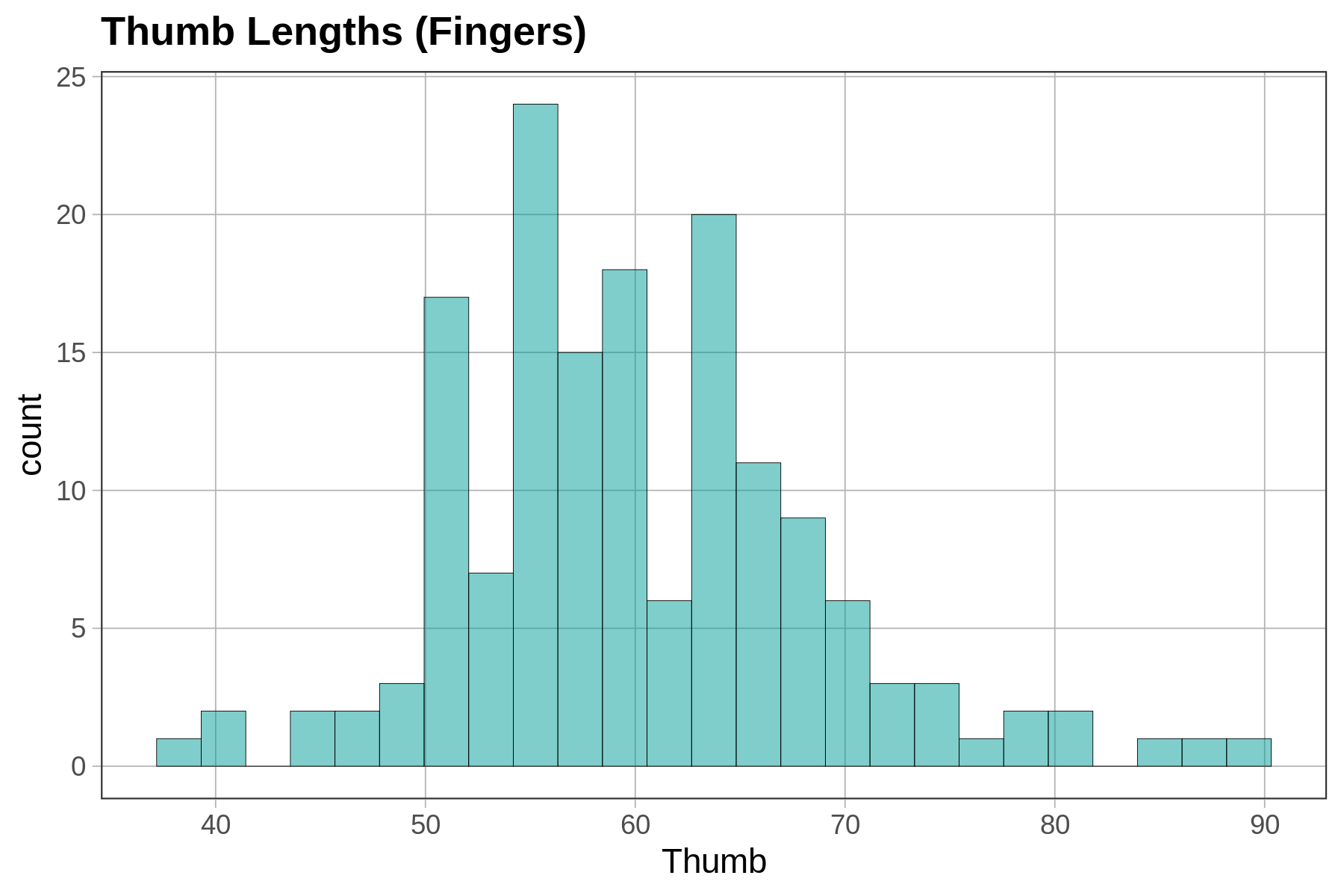
Variable 2: Thumb Lengths in the Fingers Data Frame
require(coursekata)
# modify this code to make a histogram of Thumb
gf_histogram()

# get the favstats for Thumb
# modify this code to make a histogram of Thumb
gf_histogram(~ Thumb, data = Fingers)

# get the favstats for Thumb
favstats(~ Thumb, data = Fingers)
ex() %>% {
  check_or(.,
    check_function(., "gf_histogram") %>% {
      check_arg(., "object") %>% check_equal()
      check_arg(., "data") %>% check_equal()
    },
    override_solution(., "gf_histogram(Fingers, ~ Thumb)") %>%
      check_function("gf_histogram") %>% {
        check_arg(., "object") %>% check_equal()
        check_arg(., "gformula") %>% check_equal()
      },
    override_solution(., "gf_histogram(~ Fingers$Thumb)") %>%
      check_function("gf_histogram") %>%
      check_arg(., "object") %>%
      check_equal()
  )
  check_function(., "favstats") %>%
    check_result() %>%
    check_equal()
}
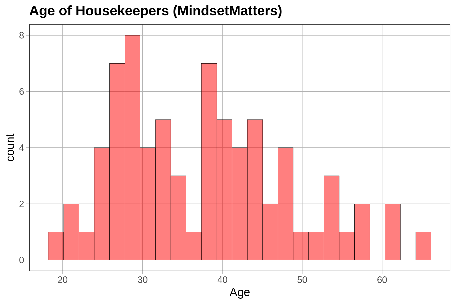
Variable 3: Age of Housekeepers in the MindsetMatters Data Frame
require(coursekata)
# make a histogram of Age in the MindsetMatters data frame
# set the fill = "red"

# get the favstats for Age
# make a histogram of Age in the MindsetMatters data frame
# set the fill = "red"
gf_histogram(~ Age, data = MindsetMatters, fill = "red")

# get the favstats for Age
favstats(~ Age, data = MindsetMatters)
ex() %>% {
  check_or(.,
    check_function(., "gf_histogram") %>% {
      check_arg(., "object") %>% check_equal()
      check_arg(., "data") %>% check_equal()
    },
    override_solution(., "gf_histogram(MindsetMatters, ~ Age)") %>%
      check_function("gf_histogram") %>% {
        check_arg(., "object") %>% check_equal()
        check_arg(., "gformula") %>% check_equal()
      },
    override_solution(., "gf_histogram(~ MindsetMatters$Age)") %>%
      check_function("gf_histogram") %>%
      check_arg(., "object") %>%
      check_equal()
  )
  check_function(., "gf_histogram") %>%
    check_arg("fill") %>%
    check_equal()
  check_function(., "favstats") %>%
    check_result() %>%
    check_equal()
}
In general, the median may be a more meaningful summary of a distribution of data than the mean, when the distribution is skewed one way or the other. In essence, this discounts the importance of the tail of the distribution, focusing more on the part of the distribution where most people score. The mean is a good summary when the distribution is more symmetrical.
But, if our goal is to create a statistical model of the population distribution, we almost always—especially in this course—will use the mean. We shall dig in a little to see why. But first, a brief detour to see how we can add the median and mean to a histogram.
Adding Median and Mean to Histograms
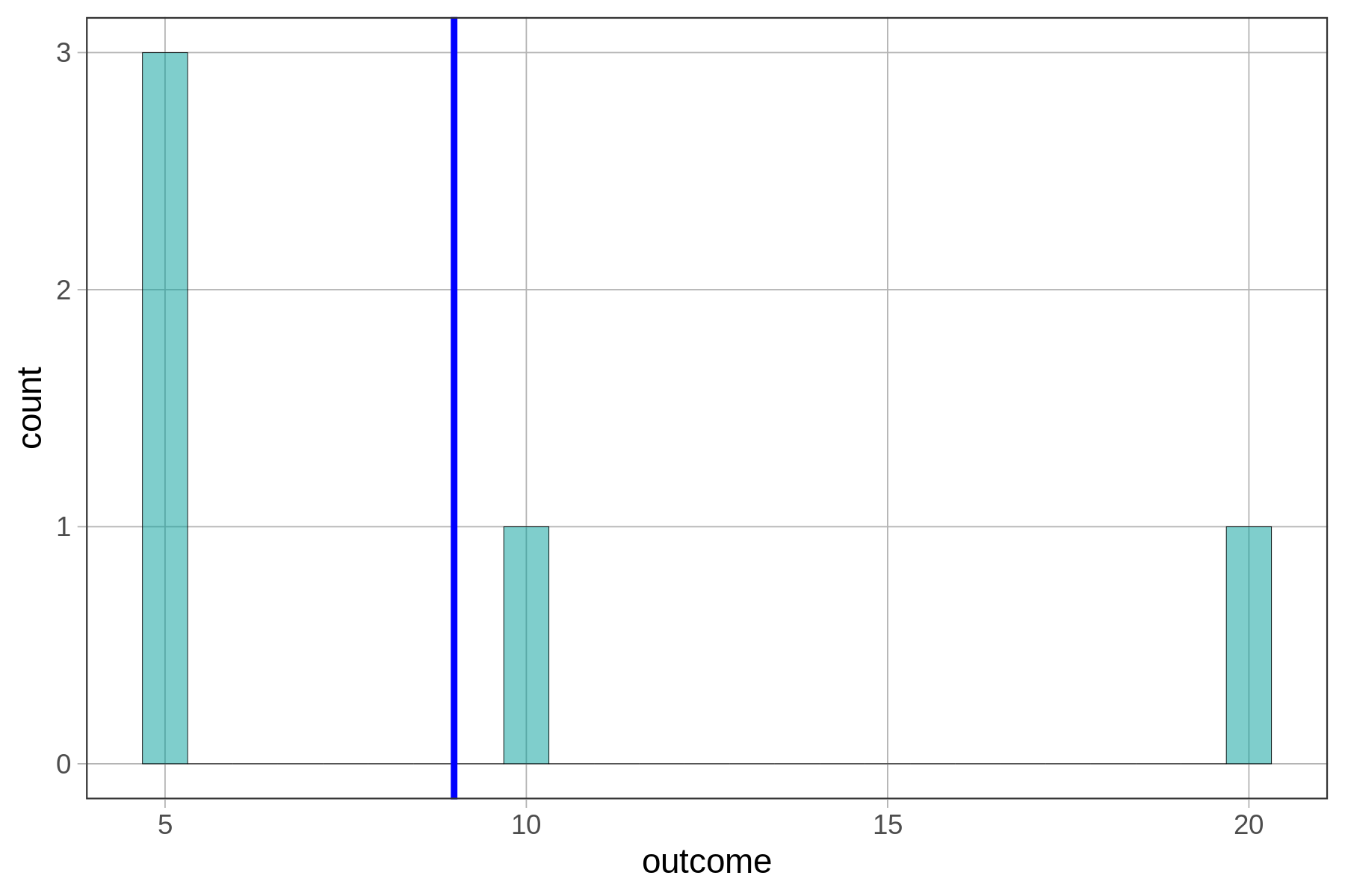
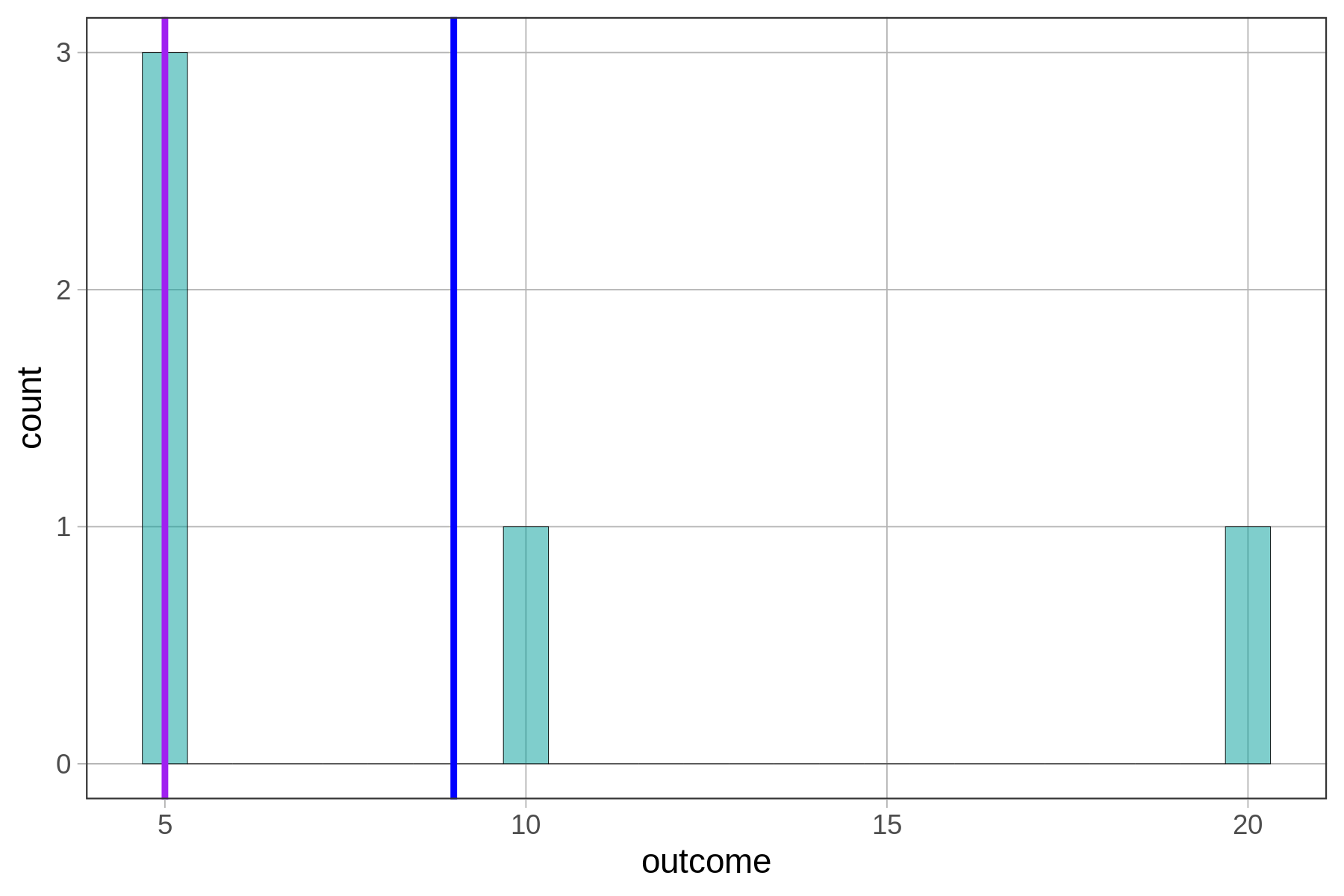
You already know the R code to make a histogram. Let’s add a vertical line to show where the mean is. We know from favstats() that the mean is 9, so we can just add a vertical line that crosses the x-axis at 9. Let’s color it blue.
gf_histogram(~ outcome) %>%
  gf_vline(xintercept = 9, color = "blue")
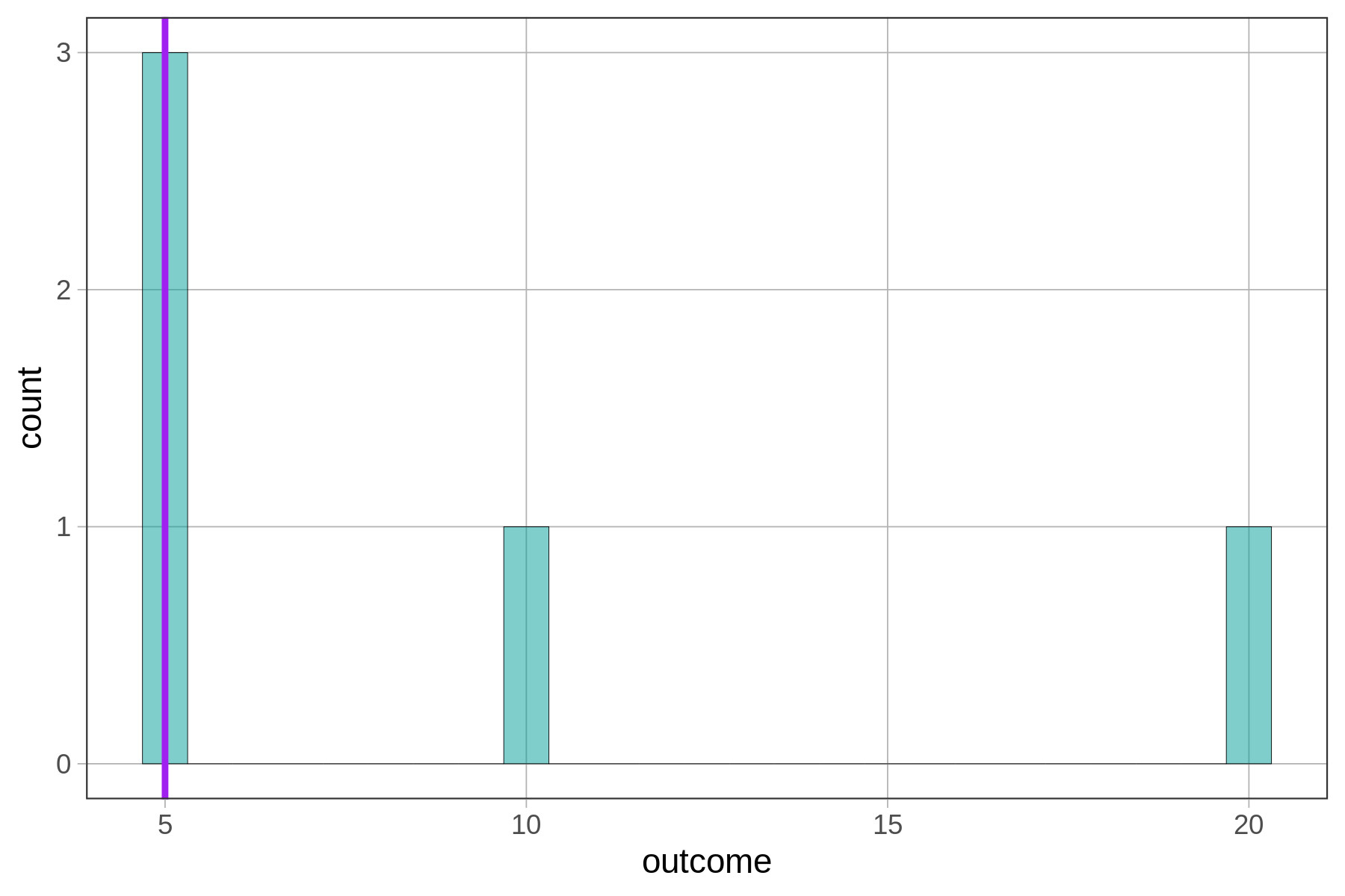
Try modifying this code to draw a purple line for the median of this tiny set of numbers. (The median is 5.)
require(coursekata)
outcome <- c(5, 5, 5, 10, 20)
# Modify this code to draw a vline representing the median in "purple"
gf_histogram(~outcome) %>%
  gf_vline(xintercept = 9, color = "blue")
# Modify this code to draw a vline representing the median in "purple"
gf_histogram(~outcome) %>%
  gf_vline(xintercept = 5, color = "purple")
ex() %>% {
  check_function(., "gf_histogram") %>%
    check_arg("object") %>%
    check_equal()
  check_function(., "gf_vline") %>% {
    check_arg(., "xintercept") %>% check_equal()
    check_arg(., "color") %>% check_equal()
  }
}
You can string these commands together (using %>%) to put both the mean and median lines onto a histogram. (This time, we used the mean() and median() functions instead of typing in the actual numbers.)
gf_histogram(~ outcome) %>%
  gf_vline(xintercept = mean(outcome), color = "blue") %>%
  gf_vline(xintercept = median(outcome), color = "purple")
Note there is a related function called gf_hline() that will place a horizontal line on a plot (it takes yintercept as an argument).