5.6 Generating Predictions From the Empty Model
The mean of the sample distribution is our best, unbiased estimate of the mean of the population. For this reason, we use the mean as our model for the population. And, if we want to predict what the next randomly sampled observation might be, without any other information, we would use the mean.
In data analysis, we also use the word “predict” in another sense and for another purpose. Using our Fingers data, we found the mean thumb length to be 60.1 mm. So, if we were predicting a new student’s thumb length, we’d go with 60.1 mm. But if we take the mean and look backwards at the data we have already collected, we could also generate a “predicted” thumb length for each of the data points we already have. This prediction answers the question: what would our model have predicted this thumb length to be if we hadn’t collected the data?
There’s an R function called predict() that will actually do this for you. Here’s how we can use it to generate the predicted thumb lengths for each of the 157 students in the Fingers data frame. Remember, we already fit the model and saved the results in empty_model:
predict(empty_model)Try using the predict() function to generate predicted thumb lengths using the empty model in the code window below.
require(coursekata)
# saves the empty model
empty_model <- lm(Thumb ~ NULL, data = Fingers)

# write code to generate predictions of the empty model
empty_model <- lm(Thumb ~ NULL, data = Fingers)
predict(empty_model)
ex() %>% check_object("empty_model") %>% check_equal()You may be wondering: why would we want to create predicted thumb lengths for these 157 students when we already know their actual thumb lengths? We will go into this a lot more in the next chapter, but briefly, the reason is so we can get a sense of how far off the model predictions are from the actual data. In other words, it gives us a rough idea of how much error there is around the model predictions, i.e., how well our model fits our current data.
In order to use these predicted scores as a way of seeing how much error there is, we first need to save the prediction for each student in the data set. When there is only one prediction for everyone, as with the empty model, it seems like overkill to save the predictions.
But as we go, we’ll start to appreciate how useful it is to save the individual predicted scores. For example, if we save the predicted score for each student in a new variable called Predict, we can then subtract each student’s actual thumb length from their predicted thumb length to see how far off the prediction is for each student.
In the code window below, use the predict() function to save the predicted thumb lengths for each of the 157 students as a new variable in the Fingers data set. We’ve added some code to overlay these predictions onto a scatterplot we’ve looked at before (Thumb by Height).
require(coursekata)
# this saves the empty_model
empty_model <- lm(Thumb ~ NULL, data = Fingers)

# modify this to save the predictions from the empty_model in a new variable
Fingers$Predict <-

# prints out selected variables from Fingers
head(select(Fingers, Thumb, Predict), 10)

# this makes a scatterplot of Thumb by Height and overlays the empty model's predictions as open blue circles
gf_point(Thumb ~ Height, data = Fingers, width = .1) %>%
  gf_point(Predict ~ Height, color = "blue", shape = 1, height = 0)
# this saves the empty_model
empty_model <- lm(Thumb ~ NULL, data = Fingers)

# modify this to save the predictions from the empty_model in a new variable
Fingers$Predict <- predict(empty_model)

# prints out selected variables from Fingers
head(select(Fingers, Thumb, Predict), 10)

# this makes a scatterplot of Thumb by Height and overlays the empty model's predictions as open blue circles
gf_point(Thumb ~ Height, data = Fingers, alpha = .2) %>%
  gf_point(Predict ~ Height, color = "blue", shape = 1)
ex() %>%
  check_object("Fingers") %>%
  check_column("Predict") %>%
  check_equal()
A snippet of the Fingers data frame
|
A scatterplot of Thumb by Height
|
|---|---|
|
|
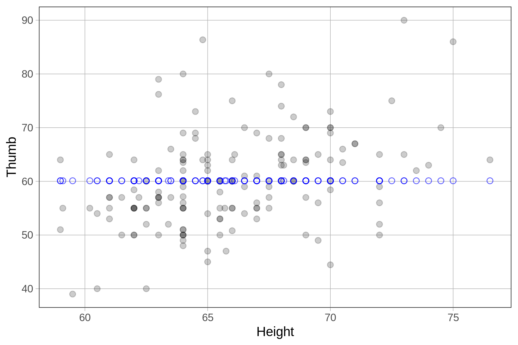
As we can see from the sample rows from the Fingers data frame (on the left), every student, regardless of their thumb length, is given the same model prediction (60.1). This is because in the empty model, there is only one prediction, and that is the mean.
In the scatterplot, we might see a relationship between Thumb and Height in the data. But the empty model ignores all that and just predicts the same thumb length for every student, which is why the predictions (Fingers$Predict) form a straight horizontal line. (Later we will learn how to adjust predictions based on explanatory variables such as sex or height).