6.3 Variance
Sum of squares is a good measure of total variation in an outcome variable if we are using the mean as a model. But, it does have one important disadvantage.
Consider these distributions.
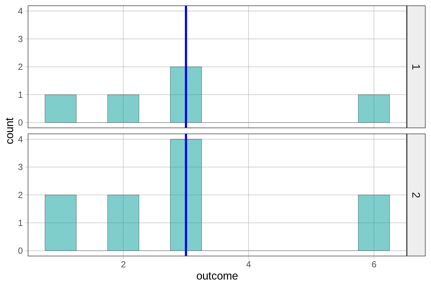
SS from Mean for distribution 1:  14
SS from Mean for distribution 2:  28
Although you can see that the spread of the data points does not look different between the two distributions, the one on the bottom (#2) has a much larger SS.
Even worse, take a look at this pair of distributions.
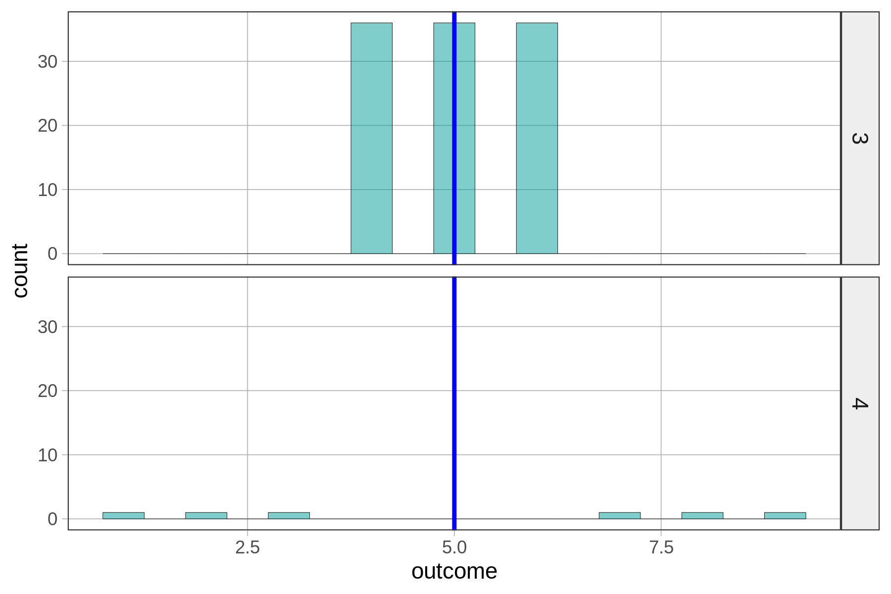
SS from Mean for distribution 3:  72
SS from Mean for distribution 4:  58
Sum of squares works fine as a way to quantify error around the mean, and compare error across two distributions, but only when both distributions have the same sample size.
The reason for this is that each time you add another data point to the sample distribution, you are adding another squared deviation from the mean to the total SS. So even if two distributions appear to be equally well modeled by their respective means, they may have very different SS. SS always grows as the number of data points in the distribution gets larger, irrespective of the degree of spread.
This problem is solved by adding two new statistics to our toolbox: variance and standard deviation. To calculate variance, we start with SS, or total error, but then divide by the sample size to end up with a measure of average error around the mean—the average of the squared deviations.
Because it is an average, variance is not impacted by sample size, and thus, can be used to compare the amount of error across two samples of different sizes. You can think of it as a measure of average variation per sampled unit (e.g., students) in the data set.
The formula for variance, usually represented as \(s^2\), is this:
\[\frac{\sum_{i=1}^n (Y_i-\bar{Y})^2}{n-1}\]
You can see that the numerator is the sum of squares. Although to get an actual average of squared deviations you would divide by n, we instead divide by n-1. We do this because dividing by n-1 gives us a better estimate of the true population variance, a fact that can be demonstrated by simulating multiple random samples from a population of known variance and then seeing which estimates are better – those obtained by dividing by n, or those obtained dividing by n-1.
There is, of course, a mathematical proof for this (for reference, here you can download mathematical proof for n-1 correction (PDF, 347KB)). But we find it helpful to think about this way: when you take a small sample, the most extreme values in a population are unlikely to show up. So, if we divided by n it would, especially in smaller samples, slightly underestimate the true population variance. Dividing by n-1 corrects this bias, making the variance estimate a bit larger. And, as the sample gets larger, the difference between n and n-1 makes less and less difference.
The main thing to know is that taking the SS and dividing by n-1 results in something that approximates an average squared deviation. (Also note: the n-1 you see in the denominator is sometimes called the degrees of freedom, or df. This will be more important later.)
To calculate variance in R we can use the var() function. Here is how to calculate the variance of our Thumb data from Fingers.
var(Fingers$Thumb)You can also find variance by running the supernova() function on the empty model. In the code window below, try using both the var() function and the supernova() function to calculate the variance of Thumb in the Fingers data frame.
require(coursekata)
empty_model <- lm(Thumb ~ NULL, data = Fingers)
# this creates the empty_model
empty_model <- lm(Thumb ~ NULL, data = Fingers)

# calculate the variance of Thumb from the Fingers data frame
var()

# use supernova() on the empty_model to calculate variance
supernova()
var(Fingers$Thumb)
supernova(empty_model)
ex() %>% check_function("var") %>% check_result() %>% check_equal()
ex() %>% check_function("supernova") %>% check_result() %>% check_equal()76.1551981994121Analysis of Variance Table (Type III SS)
Model: Thumb ~ NULL
SS df MS F PRE p
----- ----------------- --------- --- ------ --- --- ---
Model (error reduced) | --- --- --- --- --- ---
Error (from model) | --- --- --- --- --- ---
----- ----------------- --------- --- ------ --- --- ---
Total (empty model) | 11880.211 156
You can see that the variance of Thumb is the same, whether produced by the var() function or the supernova() function. In the ANOVA table, however, variance goes by a different name: MS. MS stands for Mean Square, as in the “mean of the sum of squares.” If you divide the sum of squares (11880.211) by n-1 (156), you will also get the MS, or variance, of 76.155.