Chapter 15 - Models with Interactions

15.1 Dogs in the Emergency Room

In previous chapters we introduced models with multiple predictor variables, and used these models to produce better predictions, with less error (usually), than we were able to achieve with single-predictor models. In this chapter we add one more twist to the story. All the multivariate models we have built so far are additive. In this chapter we will explain what that means, and then learn how to add interactions to our models.

Anxiety in the Emergency Room

Going to the emergency room can be an ordeal that provokes a lot of anxiety. Being sick or injured, then having to wait, can make people feel quite anxious, which probably isn’t very good for patients’ overall health. In this chapter we will analyze some data produced by a group of researchers trying to figure out how they might reduce anxiety among patients who come to the ER.

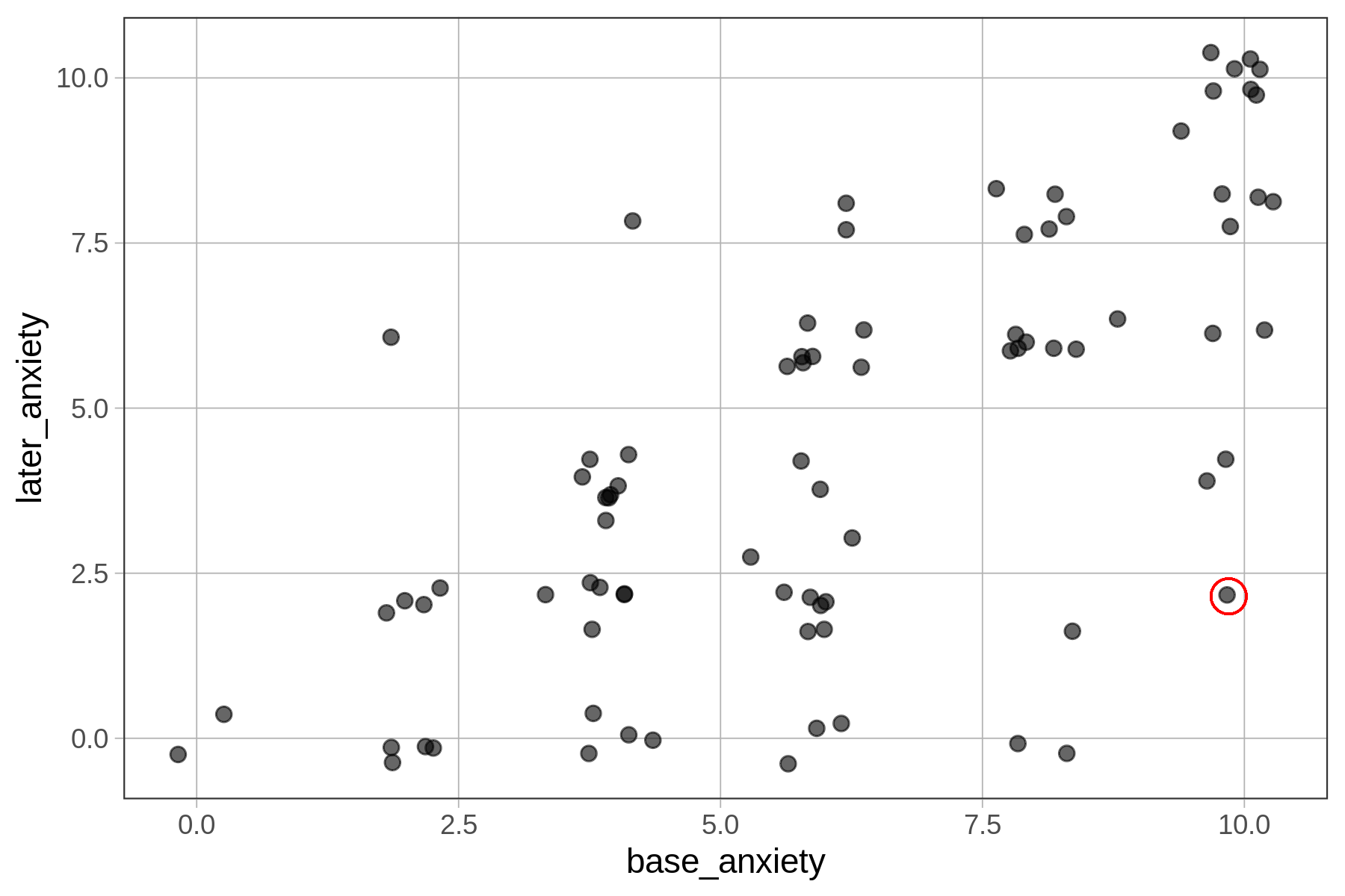
The data frame er includes data from 84 patients who came to the emergency room and who were initially identified by ER personnel as appearing to exhibit some anxiety. Patients included in the study were asked to rate their own level of anxiety, on a scale of 1 to 10 twice: once on initial entry into the ER (base_anxiety) and then again 30 minutes later (later_anxiety).

Here’s a jitter plot that shows later_anxiety as a function of base_anxiety.

gf_jitter(later_anxiety ~ base_anxiety, data=er)

Could a Therapy Dog Help to Reduce Anxiety?

The data we’ve been analyzing came from a study in which patients initially identified as anxious were randomly assigned to one of two conditions on arrival at the ER. Patients in the Dog group (n=43) were given a therapy dog to spend time with while they waited to see a doctor. Patients in the Control group just waited as usual, with no access to a dog. The researchers hypothesized that therapy dogs might help to lessen patients’ anxiety as they waited.

source: https://www.barringtonbhw.com/the-benefits-of-therapy-dogs/

Add the color argument into the jitter plot to color the dots according to which condition each patient was assigned to (hint: there is a ~ involved).

Fitting the Additive Model

In the previous chapters we learned to fit these types of multivariate models; we will now start referring to them as additive or main effects models. Let’s look at the later_anxiety = condition + base_anxiety + other stuff model to see why it is called an additive model.

In the code window below, fit the multivariate model represented by this word equation (later anxiety = condition + base anxiety + other stuff) to the er data set. Save the model as additive_model, then print out the ANOVA table.

Analysis of Variance Table (Type III SS)
Model: later_anxiety ~ condition + base_anxiety

                                     SS df      MS      F    PRE     p
 ------------ --------------- | ------- -- ------- ------ ------ -----
        Model (error reduced) | 469.512  2 234.756 51.147 0.5581 .0000
    condition                 |  85.790  1  85.790 18.691 0.1875 .0000
 base_anxiety                 | 409.948  1 409.948 89.317 0.5244 .0000
        Error (from model)    | 371.774 81   4.590
 ------------ --------------- | ------- -- ------- ------ ------ -----
        Total (empty model)   | 841.286 83  10.136

Visualizing and Interpreting the Additive Model

In the scatter plot below we have overlaid the additive model using this code:

gf_jitter(later_anxiety ~ base_anxiety, color = ~condition, data = er) %>%
gf_model(additive_model)

Use the code window below to print out the best-fitting parameter estimates of the additive model.

Call:
lm(formula = later_anxiety ~ condition + base_anxiety, data = er)

Coefficients:
 (Intercept)  conditionDog  base_anxiety
      0.4317       -2.0279        0.8112