3.11 The Back and Forth Between Data and the DGP
Data analysis involves working back-and-forth between the data distribution, on one hand, and our best guess of what the population distribution looks like, on the other. We need to keep this in mind in order to understand the DGP that might have produced the variation in the population and thus the variation we see in our data.
As you learn to think like a statistician, it helps to understand the two key moves that you will use as part of this back-and-forth.
Looking at a distribution of data, you try to imagine what the population distribution might look like, and what processes might have produced such a distribution. We will call this a bottom-up strategy as we move from concrete data to the more unknown, abstract DGP.
Thinking about the DGP, and all that you know about the world, you try to imagine what the data distribution should look like, if your theory of the DGP is true. We will call this the top-down strategy as we move from our ideas about the DGP to predicting actual data.
We illustrated the bottom-up move above when we looked at the distribution of wait times at a bus stop and tried to imagine the process that generated it. The top-down move would come into play if we asked: what if buses worked differently? What if, instead of following schedules, a new bus left the stop every time 10 people were waiting there? What would the distribution of wait times look like if this were the case?
You can probably imagine a few different possibilities. That’s great! Having some expectations about the DGP (whether they are right or wrong) can help us interpret any data that we actually do collect.
Both the top-down and bottom-up moves are important. Sometimes we have no clue what the DGP is, so we have no choice but to use the bottom-up strategy, looking for clues in the data. Based on these clues, we generate hypotheses about the DGP.
But other times, we have some well-formulated ideas of the DGP that we can test by looking at the data distribution. In the top-down move we say: if our theory is correct, what should the data distribution look like? If it looks like we predict, our theory is supported. But if it doesn’t, we can be pretty sure we are wrong about the DGP.
When We Know the DGP: The Case of Rolling Dice
Our understanding of the DGP is often fuzzy, imperfect, and sometimes flat out wrong. But some DGPs are well-known, such as coin flips and dice rolls, which are purely random processes.
Randomness turns out to be an important DGP for the field of statistics. We often question whether the distribution in our data could result from purely random processes. We can start to answer this question by taking a top-down approach: imagining a purely random process and examining the various distributions of data it could produce.
Dice provide a familiar model for thinking about random processes. They also provide a useful example for thinking about the related concepts of sample, population, and DGP. In most research, we are trying to understand DGPs we don’t already know, so we can only engage in bottom-up thinking, starting with a sample and trying to guess what the DGP might be like. With dice we have the luxury of going top-down, starting with the DGP, simply because we know what the DGP is.
Using R to Make a DGP
We could explore the DGP of rolling dice by just rolling them thousands of times. But luckily we don’t have to do this. We can, instead, use R to “roll dice” for us, not just one time but many times. If we let our program to simulated dice rolls run for a long time, we can see what the population distribution would look like.
Let’s start by programming up a DGP that would randomly generate a whole number between 1 and 6. In essence, this is what a dice roll is: a random process that picks one of the 6 possible numbers on a dice. To simulate this process in R, we can start by making a vector with the numbers 1 through 6.
dice_outcomes <- c(1, 2, 3, 4, 5, 6)Like an actual dice, the vector dice_outcomes contains each number from 1 to 6. By randomly sampling from this vector, we can simulate the DGP of rolling dice. To simulate a single roll of the dice, we can run this line of R code:
sample(dice_outcomes, 1)This tells R to randomly sample one number from the numbers in dice_outcomes, of which there are six. If we run the sample() function, it will return a vector with a single value in it. For example, we ran it just now and got the following output. Turns out our simulated dice rolled a 2 this time.
[1] 2Try using this DGP in the code block below.
require(coursekata);
dice_outcomes <- c(1, 2, 3, 4, 5, 6)

# edit this code to simulate one dice roll
# and to save it in a vector called my_sample
my_sample <- sample()

# print out my_sample
dice_outcomes <- c(1, 2, 3, 4, 5, 6)

# edit this code to simulate one dice roll
# and to save it in a vector called my_sample
my_sample <- sample(dice_outcomes, 1)

# print out my_sample
my_sample
ex() %>% {
    override_solution_code(.,
        'dice_outcomes <- c(1, 2, 3, 4, 5, 6); my_sample <- sample(dice_outcomes, 1); my_sample'
    )
    }
Try running your dice roll simulation code a few times. Why does it come up with these particular numbers? The answer to this question would be, “It’s just randomness.” Even if your simulated dice rolling DGP produced a surprising pattern (e.g., five 1s in a row), the explanation would still be, “It’s just randomness.” We can say this because we created the DGP ourselves using R and we know what it is!
What do we mean when we say “randomness”? A random process is one where individual events are unpredictable, even though the long term probabilities of different events are known. In the case of dice, we cannot predict which number will be rolled on any particular occasion. However, we do know that each of the numbers 1 to 6 has an equal likelihood of being rolled over the long run.
The bar graph below represents this idea with a uniform probability distribution. The the probability of a particular number being rolled would be \(\frac{1}{6}\) or \(0.1\bar{6}\).
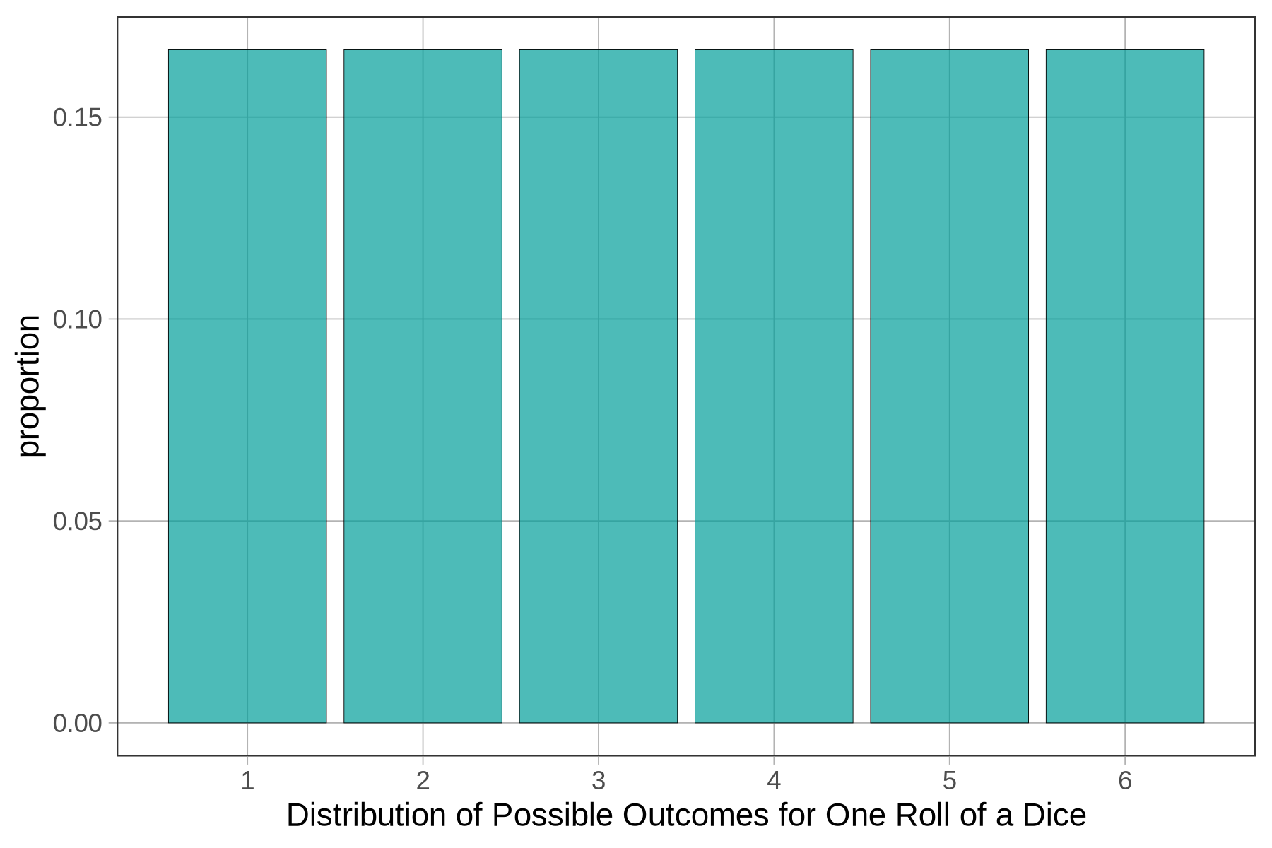
Theoretically, if we were to run this DGP of dice rolling many times (thousands!), we would end up with a population distribution similar to the graph above.
(Note that although the graph looks like a histogram it is not. We use gf_bar() instead of gf_histogram() because the outcomes of rolling a dice are categorical, not quantitative. The numbers 1 to 6 are not, in this case, measurements of some continuous variable but just the names of 6 possible results.)