12.11 Confidence Interval for the Slope of a Regression Line

Let’s go back to the regression model we fit using total Check to predict Tip. We can specify this model of the DGP like this:

$$Y_i={\beta }_0+{\beta }_1{X}_i+{ϵ}_i$$

Here is the output for the best-fitting Check model using lm().

Call:
lm(formula = Tip ~ Check, data = TipExperiment)

Coefficients:
(Intercept)        Check
   18.74805      0.05074

Use the code window below to find the confidence interval for the slope of this regression line.

                 2.5 %      97.5 %
(Intercept) 12.76280568 24.73328496
Check        0.02716385  0.07431286

The ${\beta }_1$ represents the increment that is added to the predicted tip in the DGP for every additional dollar spent on the total check. The confidence interval of ${\beta }_1$ represents the range of ${\beta }_1$s that would be likely to produce the sample $b_1$. About 3 cents is the lowest ${\beta }_1$ that would be likely to produce the sample $b_1$ and 7 cents is the highest.

Now that we have tried confint(), try using the resample() function to bootstrap the 95% confidence interval for the slope of the regression line. See how your bootstrapped confidence interval compares to the results obtained by using confint().

Here is a histogram of the bootstrapped sampling distribution we created. Yours will be a little different, of course, because it is random.

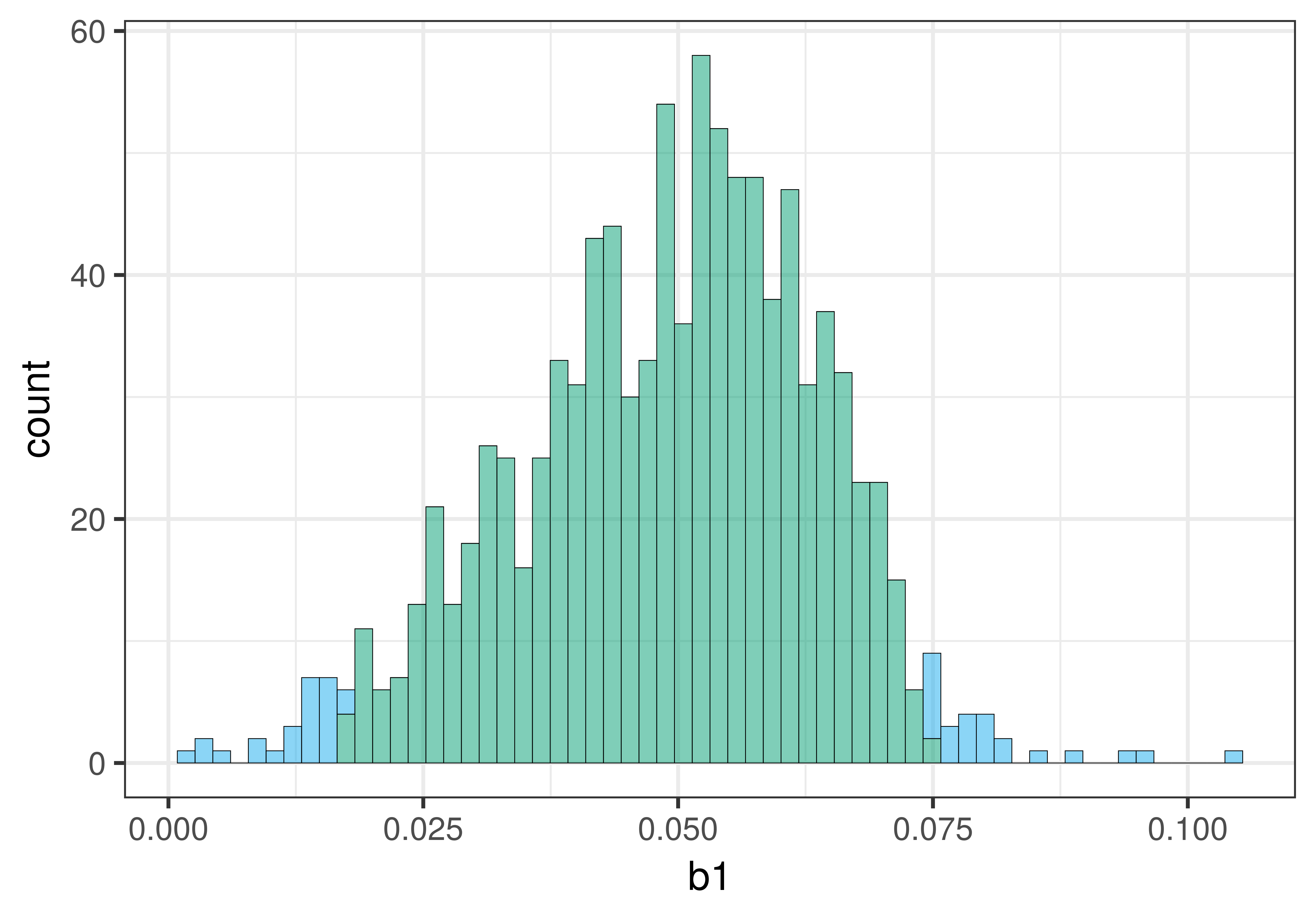
The center of the bootstrapped sampling distribution is approximately the same as the sample $b_1$ of .05. This is what we would expect because bootstrapping assumes that the sample is representative of the DGP.

As explained previously, we can use the .025 cutoffs that separate the unlikely tails from the likely middle of the sampling distribution as a handy way to find the lower and upper bound of the 95% confidence interval. We can eyeball these cutoffs by looking at the histogram, or we can calculate them by arranging the bootstrapped sampling distribution to find the actual 26th and 975th b1s.

0.0172834762542693
0.0757609233182571

To find the confidence interval, we sorted the randomly generated $b_1$s from lowest to highest, and then used the 26th and 975th $b_1$s as the lower and upper bounds of the confidence interval. Your results will be a little different from ours because resampling is random. We got a bootstrapped confidence interval of .02 to .07, which is close to what we got from confint() (.027 and .074).

The bootstrapped sampling distribution of slopes in this case is not exactly symmetrical; it is a bit skewed to the right. For this reason, the center of the confidence interval will not be exactly at the sample $b_1$. This is in contrast to the mathematical approach that assumes that the sample $b_1$ is exactly in the middle of a perfectly symmetrical t-distribution. This difference does not mean that bootstrapping is less accurate. It might be that there is something about the distributions of Check and Tip that results in this asymmetry.

The important thing we want to focus on for now is that all of these methods result in approximately the same results. These similarities show us what confidence intervals mean and what they can tell us. Later, in more advanced courses, you can take up the question of why the results differ across methods when they do.