12.2 What You have Learned about Evaluating Models
Wow, look at what you have accomplished! You can come up with questions and hypotheses, fit models, and use fancy statistics like PRE and F in order to quantify how well a model does at explaining variation. But wait—you can do even more!
Our model is the best-fitting model for our data. But what we really want to know is this: Is there really a relationship between income and hate crimes in the Data Generating Process? After all, in any given year, month, or even week, the rate of hate crimes will change and incomes are constantly changing as well. Is this relationship true in the DGP? Or was the relationship in our sample possibly just caused by random chance?
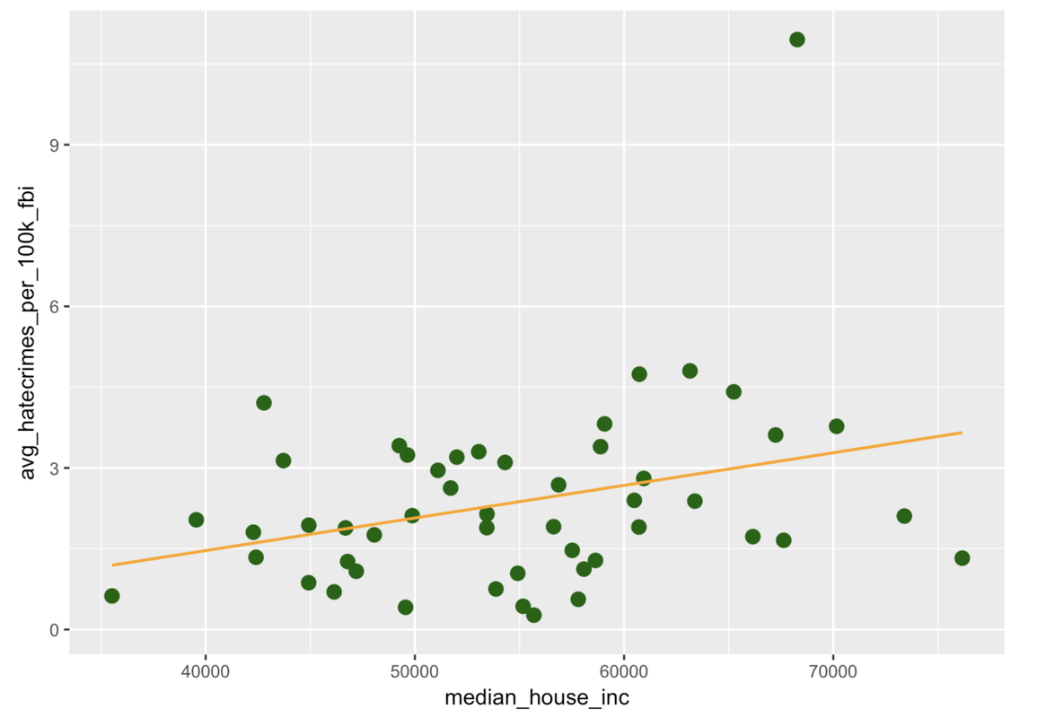
Let’s consider our relatively better model, the income model of hate crimes. Is it really better than the empty model? Is our PRE of .10 significantly higher than we would expect if there were no relationship between income and hate crimes in the DGP?
You now know how to evaluate the income model compared to the empty model. More specifically, you know how to ask whether the relationship we observed between income and hate crimes is truly present in the DGP, or whether it could simply have come about by chance, a result of random sampling variation. It turns out that everything you need to know is right in the supernova table!
Analysis of Variance Table (Type III SS)
Model: avg_hatecrimes_per_100k_fbi ~ median_house_inc

                             SS df     MS     F    PRE     p
----- --------------- | ------- -- ------ ----- ------ -----
Model (error reduced) |  14.584  1 14.584 5.409 0.1013 .0243
Error (from model)    | 129.409 48  2.696
----- --------------- | ------- -- ------ ----- ------ -----
Total (empty model)   | 143.993 49  2.939
You now know how to imagine, and instantiate in R, a world where there is no relationship between income and hate crimes! You understand the concept of sampling distribution, and you know something about what supernova() was doing in order to calculate a p of .02.
But you learned how to do much more than just read and interpret the p-value in the supernova table. You also learned how to use different techniques for creating sampling distributions—techniques such as bootstrapping, randomization, and simulation.
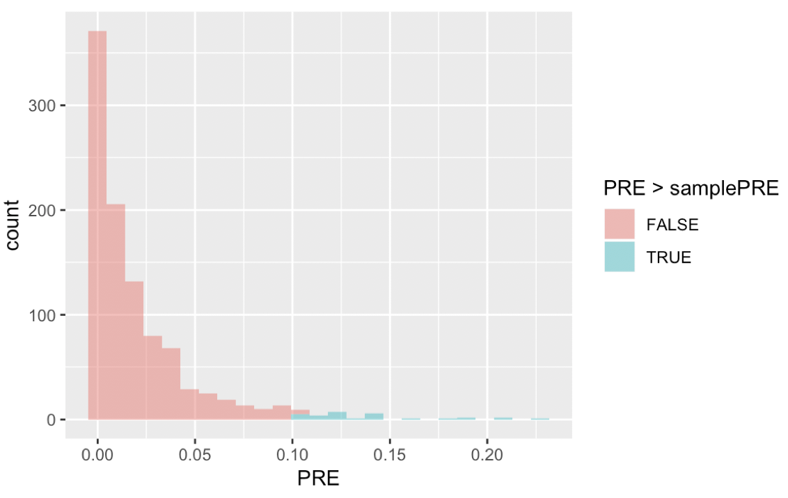
Let’s use randomization to replicate what we found in the supernova table. To start, let’s create a sampling distribution with 1,000 randomized PREs. We’ve written code in the code window below to fit the linear model to our sample, and save the sample PRE as samplePRE.
Add code to get 1,000 randomized samples (using shuffle()), and save their PREs in a data frame. Then plot the sampling distribution in a histogram and fill the PREs greater than our sample PRE in a different color. Finally, run a tally() to find the likelihood of getting a PRE greater than our sample statistic just by chance (it might be helpful to get the format in “proportions”).
require(coursekata)
hate_crimes <- hate_crimes %>%
  filter(complete.cases(avg_hatecrimes_per_100k_fbi, median_house_inc))

set.seed(41)
# We've saved the sample PRE
sample_PRE <- PRE(avg_hatecrimes_per_100k_fbi ~ median_house_inc, data = hate_crimes)

# Create a sampling distribution of 1000 randomized PREs
SDoPRE <-

# depict the sampling distribution in a histogram


# run a tally
# We've saved the sample PRE
sample_PRE <- PRE(avg_hatecrimes_per_100k_fbi ~ median_house_inc, data = hate_crimes)

# Create a sampling distribution of 1000 randomized PREs
SDoPRE <- do(1000) * PRE(shuffle(avg_hatecrimes_per_100k_fbi) ~ median_house_inc, data = hate_crimes)

# NOTE: Best solution is:
# depict the sampling distribution in a histogram
# gf_histogram(~PRE, data = SDoPRE, fill = ~PRE > sample_PRE)
# run a tally to calculate p-value
# tally(~PRE > sample_PRE, data = SDoPRE, format = "proportion")

# This longer solution is here for scoring purposes and can be ignored.
# depict the sampling distribution in a histogram
gf_histogram(~PRE, data = SDoPRE, fill = ~PRE > PRE(avg_hatecrimes_per_100k_fbi ~ median_house_inc, data = hate_crimes))
# run a tally to calculate p-value
tally(~PRE > PRE(avg_hatecrimes_per_100k_fbi ~ median_house_inc, data = hate_crimes), data = SDoPRE, format = "proportion")
eq_fun <- function(x, y) (formula(x) == ~PRE > PRE(avg_hatecrimes_per_100k_fbi ~ median_house_inc, data = hate_crimes))

ex() %>% {
  check_function(., "do")
  check_function(., "PRE", index = 2)
}

ex() %>% check_or(
  check_function(., "gf_histogram") %>% {
    check_arg(., "data") %>% check_equal()
    check_arg(., "object") %>% check_equal()
    check_arg(., "fill") %>% check_equal(eval = FALSE, eq_fun = eq_fun)
  },
  override_solution(., "gf_histogram(~PRE, data = SDoPRE, fill = ~PRE > sample_PRE)") %>%
    check_function("gf_histogram") %>%
    check_arg("fill") %>% check_equal(eval = FALSE, eq_fun = function (x,y) (formula(x) == ~PRE > sample_PRE))
)

ex() %>% check_or(
  check_function(., "tally") %>% {
    check_arg(., "data") %>% check_equal()
    check_arg(., "format") %>% check_equal()
    check_arg(., "x") %>% check_equal(eval = FALSE, eq_fun = eq_fun)
  },
  override_solution(., 'tally(~PRE > sample_PRE, data = SDoPRE, format = "proportion")') %>%
  check_function("tally") %>%
  check_arg("x") %>% check_equal(eval = FALSE, eq_fun = function(x,y) (formula(x) == ~PRE > sample_PRE))
)
PRE > samplePRE
TRUE FALSE
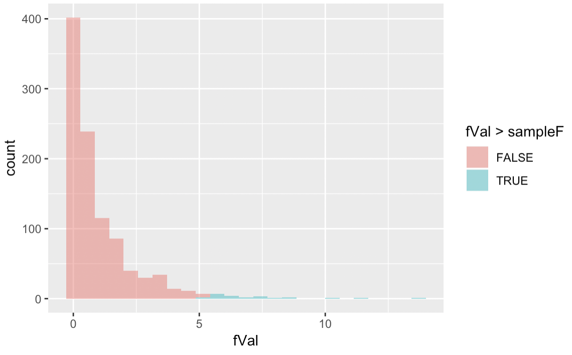
0.023 0.977You also know how to use randomization to generate a sampling distribution of F ratios, just like you did for PRE. Use the code window below to create a randomized sampling distribution of 1,000 Fs, and then calculate the probability that the F we observed in our sample could have been generated if the empty model is true.
require(coursekata)
hate_crimes <- hate_crimes %>%
  filter(complete.cases(avg_hatecrimes_per_100k_fbi, median_house_inc))

set.seed(41)
# we've saved the sample F
sample_F <- fVal(avg_hatecrimes_per_100k_fbi ~ median_house_inc, data = hate_crimes)

# create sampling distribution of randomized Fs
SDoF <-

# depict the sampling distribution in a histogram


# run a tally
# We've saved the sample F
sample_F <- fVal(avg_hatecrimes_per_100k_fbi ~ median_house_inc, data = hate_crimes)

# Create sampling distribution of randomized Fs
SDoF <- do(10) * fVal(shuffle(avg_hatecrimes_per_100k_fbi) ~ median_house_inc, data = hate_crimes)

# NOTE: Best solution is:
# depict the sampling distribution in a histogram
# gf_histogram(~fVal, data = SDoF, fill = ~fVal > sample_F)
# run a tally to calculate p-value
# tally(~fVal > sample_F, data = SDoF, format = "proportion")

# This longer solution is there for scoring purposes and can be ignored.
# depict the sampling distribution in a histogram
gf_histogram(~fVal, data = SDoF, fill = ~fVal > fVal(avg_hatecrimes_per_100k_fbi ~ median_house_inc, data = hate_crimes))
# run a tally to calculate p-value
tally(~fVal > fVal(avg_hatecrimes_per_100k_fbi ~ median_house_inc, data = hate_crimes), data = SDoF, format = "proportion")
eq_fun <- function(x, y) (formula(x) == ~fVal > fVal(avg_hatecrimes_per_100k_fbi ~ median_house_inc, data = hate_crimes))

ex() %>% {
  check_function(., "do")
  check_function(., "fVal", index = 2)
}

ex() %>% check_or(
  check_function(., "gf_histogram") %>% {
    check_arg(., "data") %>% check_equal()
    check_arg(., "object") %>% check_equal()
    check_arg(., "fill") %>% check_equal(eval = FALSE, eq_fun = eq_fun)
  },
  override_solution(., "gf_histogram(~fVal, data = SDoF, fill = ~fVal > sample_F)") %>%
    check_function("gf_histogram") %>%
    check_arg("fill") %>% check_equal(eval = FALSE, eq_fun = function(x,y) (formula(x) == ~fVal > sample_F))
)

ex() %>% check_or(
  check_function(., "tally") %>% {
    check_arg(., "data") %>% check_equal()
    check_arg(., "format") %>% check_equal()
    check_arg(., "x") %>% check_equal(eval = FALSE, eq_fun = eq_fun)
  },
  override_solution(., 'tally(~fVal > sample_F, data = SDoF, format = "proportion")') %>%
    check_function("tally") %>%
    check_arg("x") %>% check_equal(eval = FALSE, eq_fun = function(x,y) (formula(x) == ~fVal > sample_F))
)
fVal > sampleF
 TRUE FALSE
0.023 0.977
Pretty amazing. We started with a mere sample, a brief glimpse of what the Data Generating Process of hate crimes might be. But you showed that there is only a small likelihood (.02) of generating our PRE and F ratio if there is no relationship between income and hate crimes in the world. It’s an amazing thing that you can now take a sample and have sophisticated tools to say something about the population!
But we always want you to stay humble about your statistical know-how. Remember, there are always limits to what you can learn from statistics.
Closing Words
At the beginning of this course we told you that exploring variation, modeling variation, and evaluating models organizes pretty much everything you need to know about statistics. You have truly come a long way since you first heard these vague ideas. You have just demonstrated how much you have grown your statistical skills and understanding! Look at you, asking important questions with data, making amazing plots with just a few keystrokes, fitting models, using fancy GLM notation, creating sampling distributions, and interpreting your analyses with humility. Thank you for all your efforts in grappling with hard concepts. We hope you continue to pursue real understanding in this topic and beyond!