11.6 What Affects the Width of the Confidence Interval

Because our goal is to gain a more accurate picture of the DGP, it would be better to have a narrower confidence interval than a wider one. If the interval is narrower, then we will have less uncertainty in our parameter estimate, and we can make more accurate predictions about future samples. For this reason, it’s worth thinking for a bit about what determines the width of the confidence interval.

Level of Confidence

We’ve focused a lot on an alpha of .05 (when evaluating the empty model or null hypothesis), and on the corresponding 95% confidence interval. Hopefully we’ve convinced you that those two go together. But .05 and 95% are not the only criteria we could use. We could have a 99% or 90% confidence interval, or any other level.

The desired level of confidence will affect the width of the confidence interval. Given the same data, if we want to have more confidence that the DGP falls within a specified range, we will have to make our confidence interval wider.

Consider this extreme example: if we want to be 100% confident that the true value of ${\beta }_1$ falls within the confidence interval, we would need the interval to go from negative infinity to positive infinity – as wide as a confidence interval possibly could be! That’s the only way we could have 100% confidence. If we want just 95% confidence, we could make the interval narrower (whew!). And if we want even less confidence (e.g., 90% or 80%), the interval could get even narrower.

The more confidence we want (99%), the wider the interval will have to be. But how much wider?

Using confint() For Different Confidence Levels

You can use the confint() function to calculate the 90% or 99% confidence intervals (or any other level of confidence) by simply adding the argument level = .90 (or .99) to the code below. (The default if you leave off this argument is .95.)

confint(Condition_model,level=.90)

Try calculating the 90% and 99% confidence interval for the Condition model’s parameters by modifying the code below. Observe: how much wider is the 99% confidence interval?

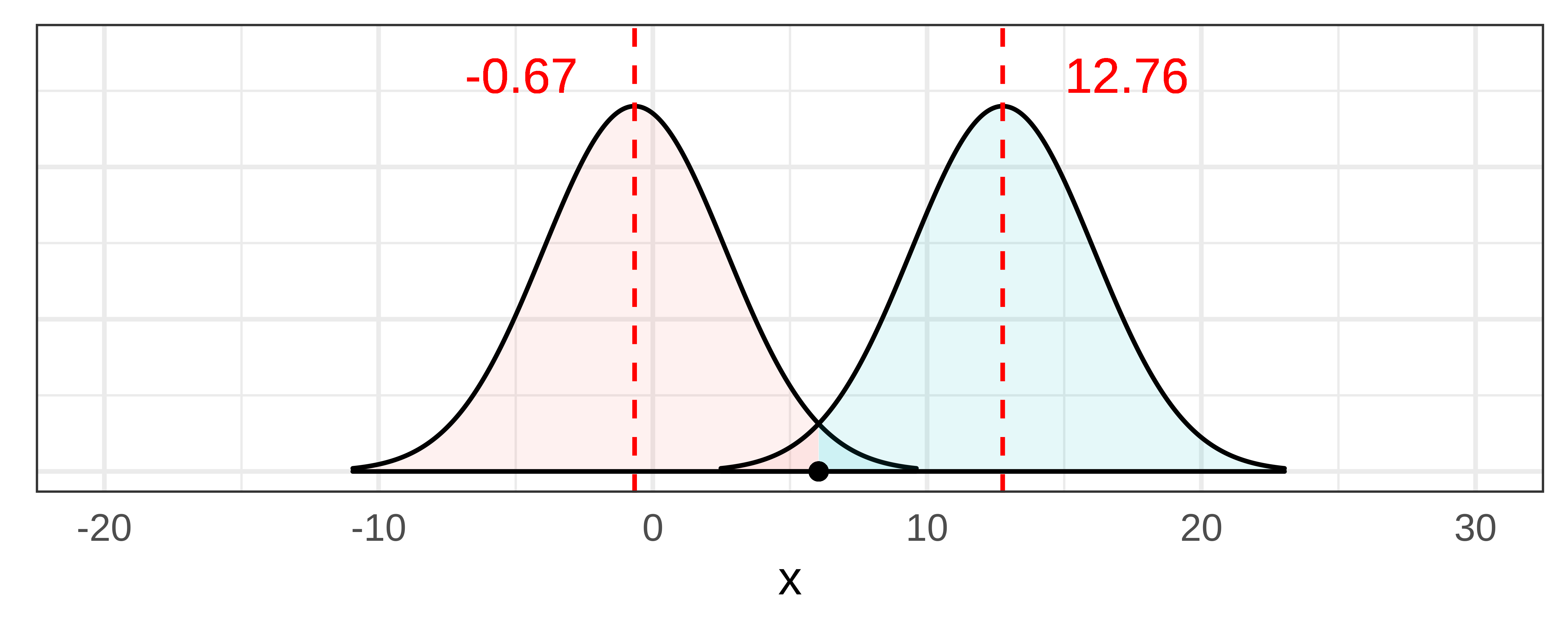
The lower bound of the 99% confidence interval is now -2.93, and the upper bound is 15.02. By increasing our confidence, we also increased the size of the confidence interval.

More Exploration of Level of Confidence and Width of the Interval

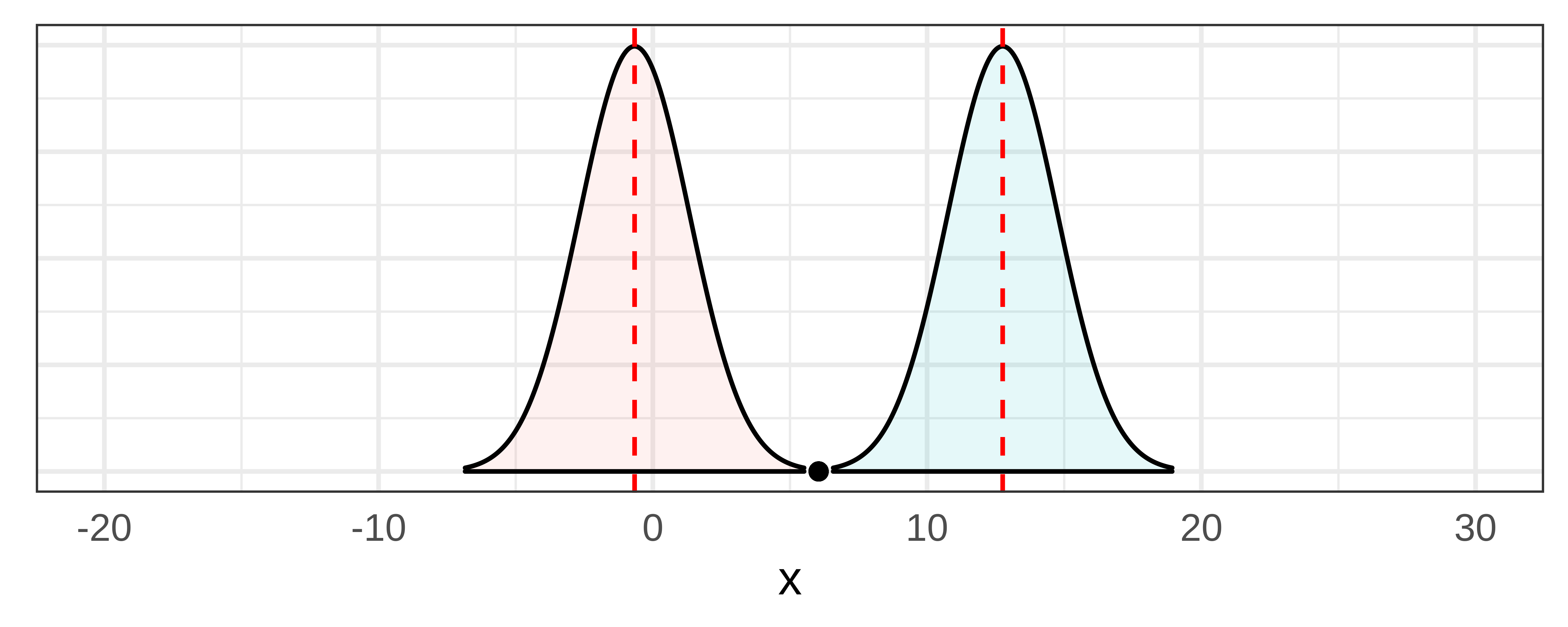
The unlikely tails are smaller in the sampling distributions used to determine the 99% confidence interval (versus the 95% one). In order to make sure the sample $b_1$ falls at the border of these smaller tails, the sampling distributions have to move farther apart.

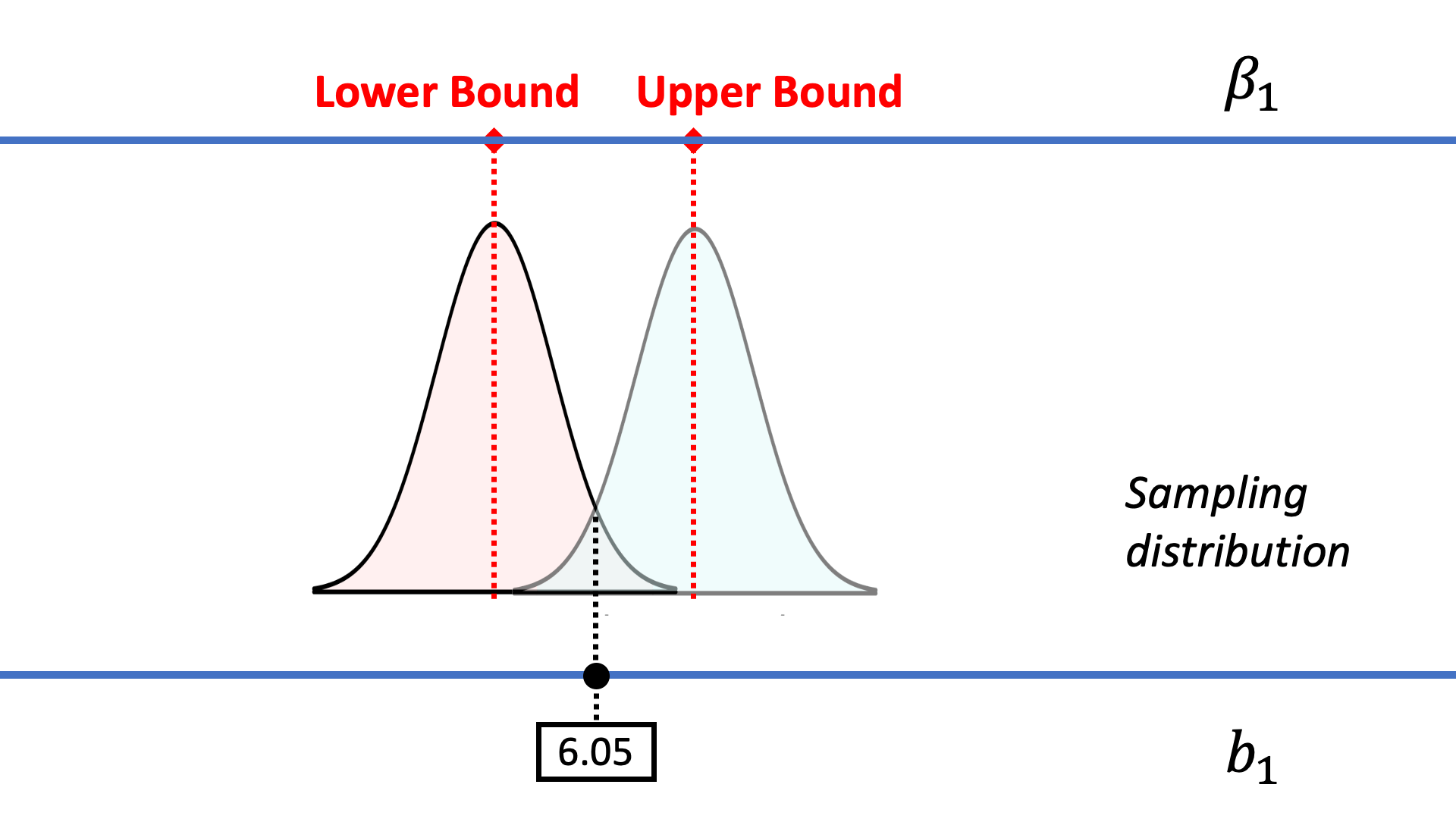
The animation above shows us that as we move the lower and upper bounds apart (thus moving their respective sampling distributions apart), the tails beyond the sample $b_1$ (the triangular shaped sections near the center of the animation) are getting smaller. This is how we get to a 99% confidence interval from a 95% one.

Let’s take a closer look at this idea by just looking at the lower bound of the confidence interval for two different levels of confidence.

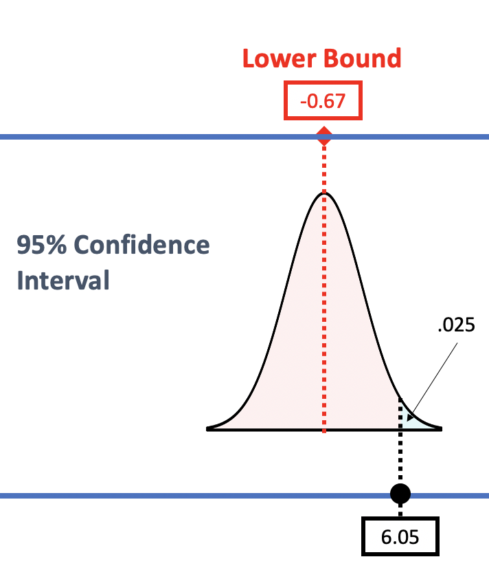
Take a look at the left panel of the figure above. To find the lower bound of the 95% confidence interval we constructed a sampling distribution and slid this sampling distribution down until we found the ${\beta }_1$ for which the sample $b_1$ would be right at the start of the .025 unlikely tail. The ${\beta }_1$ for the lower bound turned out to be -0.67; any ${\beta }_1$ lower than this would be unlikely to produce our sample (and therefore we would not include such a ${\beta }_1$ in our confidence interval).

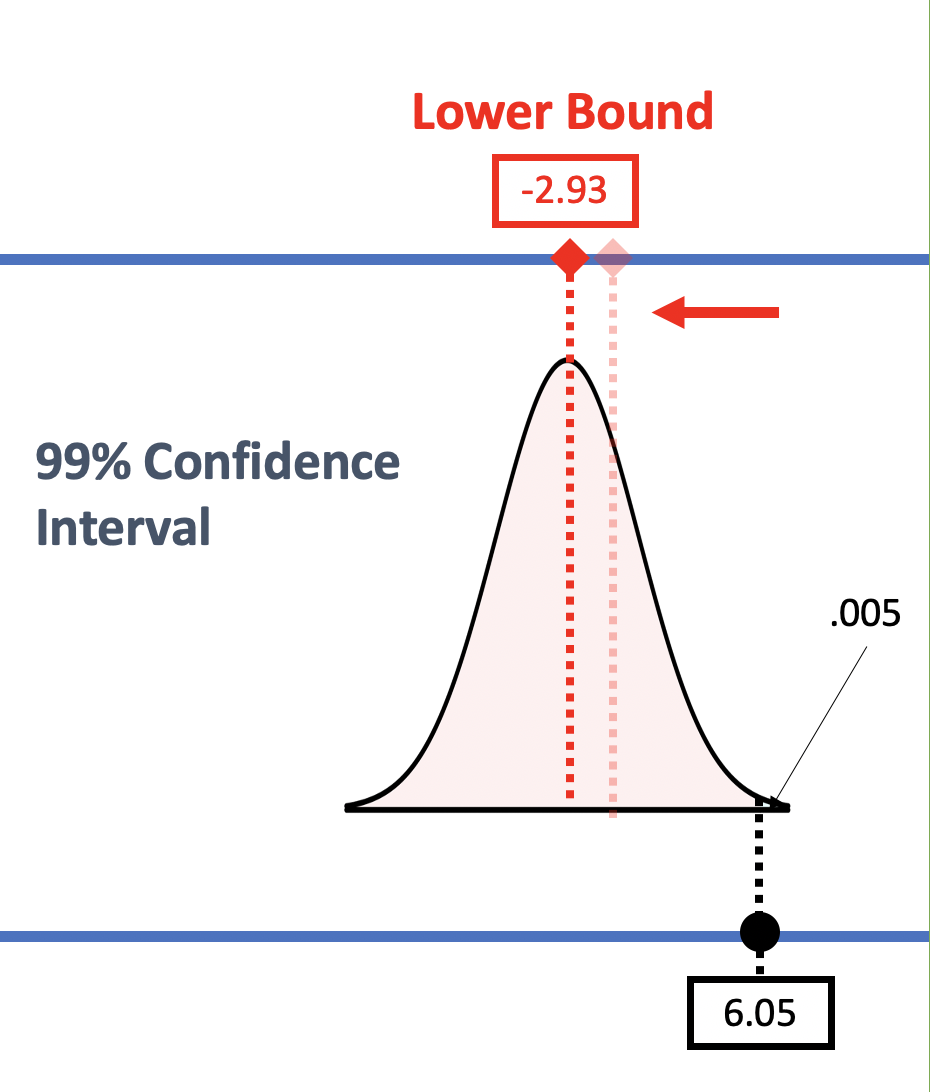
If we change the desired level of confidence to 99%, the tails that we define as unlikely will be smaller. With a smaller tail (now .005), we need to slide the sampling distribution further down (to the left) until the sample $b_1$ crosses into the unlikely region of the upper tail. As we move the sampling distribution down, the lower bound (the center of that sampling distribution) also moves down, to -2.93.

In order to go from a 95% confidence interval to a 99% interval we need to move the sampling distribution from the upper bound up and from the lower bound down thus moving the sampling distributions farther apart, making the 99% confidence interval wider relative to the 95% confidence interval.

Standard Error

Other than the level of confidence, the other factor that affects the width of the confidence interval is the standard error. The greater the standard error – i.e., the wider the sampling distribution – the wider the confidence interval will be.

We can illustrate this idea in the pictures below. In the first picture, we again have illustrated the confidence interval for ${\beta }_1$ for the Condition model in the tipping study. We constructed a sampling distribution, then moved it down and up until the sample $b_1$ crossed over into the .025 unlikely zone.

​​ Now, if we artificially make the standard error lower (e.g., revising it from 3.3 down to 2.0), you can see in the picture below that the two sampling distributions get narrower. If we don’t move their centers from the previous lower and upper bounds, you can see that the sample $b_1$ is now highly unlikely to have come from either of these narrower sampling distributions.

To find the 95% confidence interval, we want to make the sample $b_1$ fall right on the .025 cutoff. To do this we will need to slide the narrower sampling distributions closer together to the point where the sample $b_1$ just crosses over into each sampling distribution’s unlikely zone. Doing that also moves the lower and upper bounds (represented by the dotted lines) closer together.

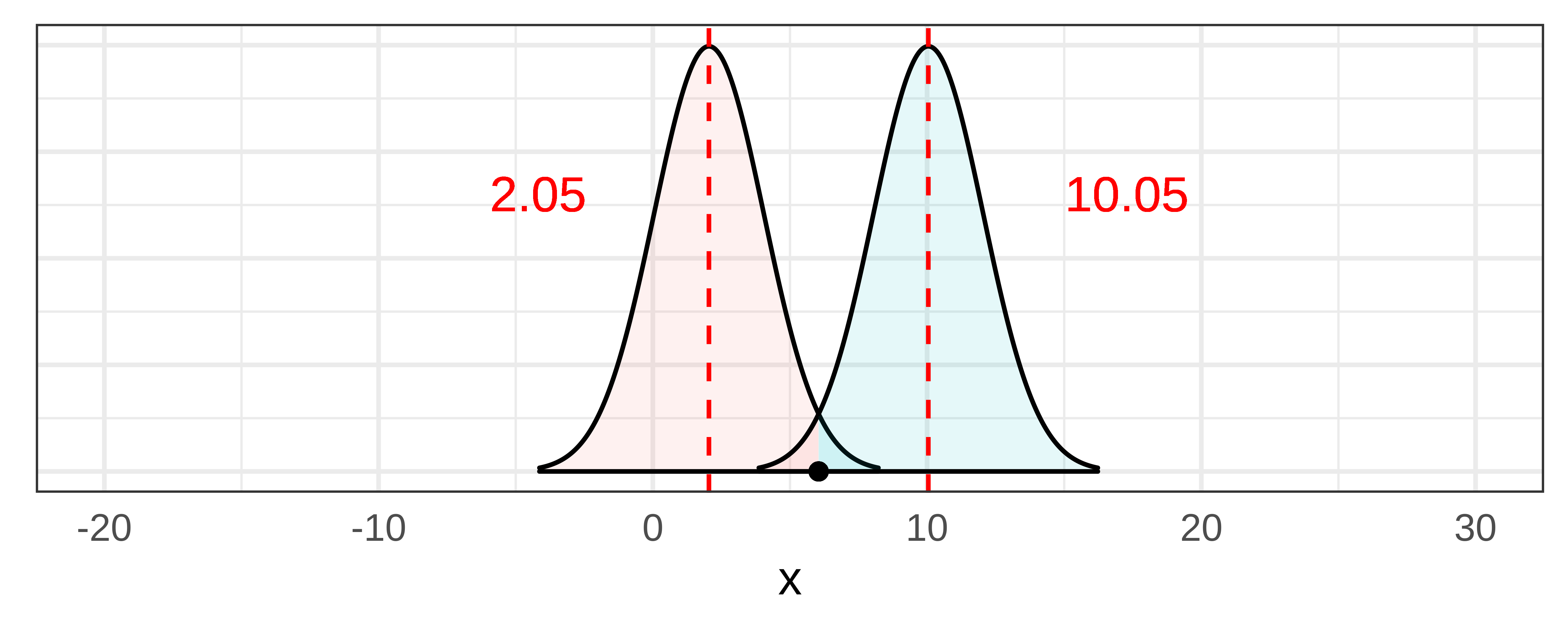
In general, therefore, as standard error gets smaller, the confidence interval gets narrower, and as standard error increases, the confidence interval gets wider.

What Affects Standard Error?

There are two things that affect standard error. One is the standard deviation of the outcome variable, in this case Tip, in the DGP. This is something you have little control over, unless you are designing the outcome measure and can make it less subject to measurement error.

The other thing that has a major effect on standard error is the sample size in the study. We’ve looked at this before when we looked at the effect of increasing the number of tables studied from n=44 to n=88. The larger the sample, the lower the standard error. For this reason, if you want less uncertainty in your estimate of ${\beta }_1$, you should try to increase the sample size in your study.

In the code window below, try your hand at calculating the 95% confidence interval for the original data with 44 tables, and for the doubled data set with 88 tables (TipExp2). We predict the one calculated from 88 tables will be narrower.

End of Chapter Survey