7.6 Graphing Residuals From the Model
You might wonder, why are we bothering to generate and save residuals? There are a lot of reasons but one short answer is: it helps us to understand the error around our model, and can suggest ways of improving the model.
Just as the first thing we do when looking at a data set is to examine the distributions of the variables, it is good to get in the habit of examining the distributions of residuals after we fit a new model.
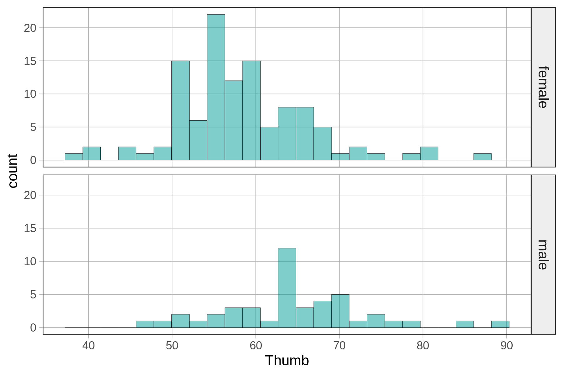
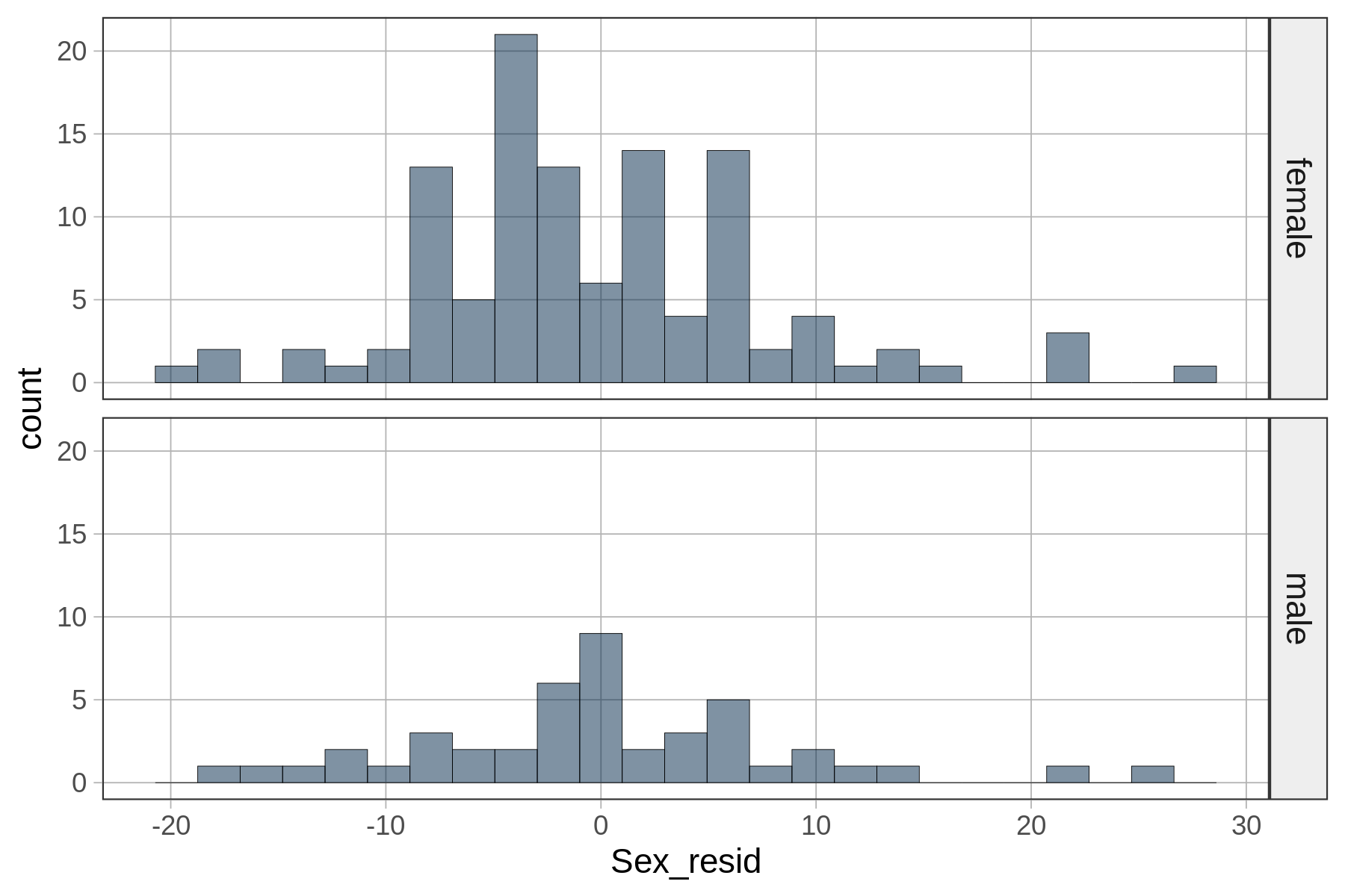
In the following window, we have provided the code to create histograms of Thumb in a facet grid by Sex. Try modifying it to generate histograms of Sex_resid in a facet grid by Sex. Compare the histograms of residuals from the Sex_model with histograms of thumb length.
require(coursekata)
# this creates the residuals from the Sex_model
Sex_model <- lm(Fingers$Thumb ~ Fingers$Sex)
Fingers$Sex_resid <- resid(Sex_model)

# this creates histograms of Thumb for each Sex
# modify it to create histograms of Sex_resid for each Sex
gf_histogram(~Thumb, data = Fingers) %>%
  gf_facet_grid(Sex ~ .)
# this creates the residuals from the Sex_model
Sex_model <- lm(Fingers$Thumb ~ Fingers$Sex)
Fingers$Sex_resid <- resid(Sex_model)

# this creates histograms of Thumb for each Sex
# modify it to create histograms of Sex_resid for each Sex
gf_histogram(~Sex_resid, data = Fingers) %>%
  gf_facet_grid(Sex ~ .)
ex() %>% {
  check_or(.,
    check_function(., "gf_histogram") %>% {
      check_arg(., "object") %>% check_equal()
      check_arg(., "data") %>% check_equal()
    },
    override_solution(., "gf_histogram(Fingers, ~ Sex_resid)") %>%
      check_function("gf_histogram") %>% {
        check_arg(., "object") %>% check_equal()
        check_arg(., "gformula") %>% check_equal()
      }
  )
  check_function(., "gf_facet_grid") %>%
    check_arg("...") %>%
    check_equal(incorrect_msg = "Make sure you keep the code to create a grid faceted by `Sex`")
}Here we’ve depicted the histograms of Thumb by Sex (in teal) next to the histograms of Sex_resid by Sex (in darker gray).
Thumb
|
Sex_resid
|
|---|---|
|
|
|
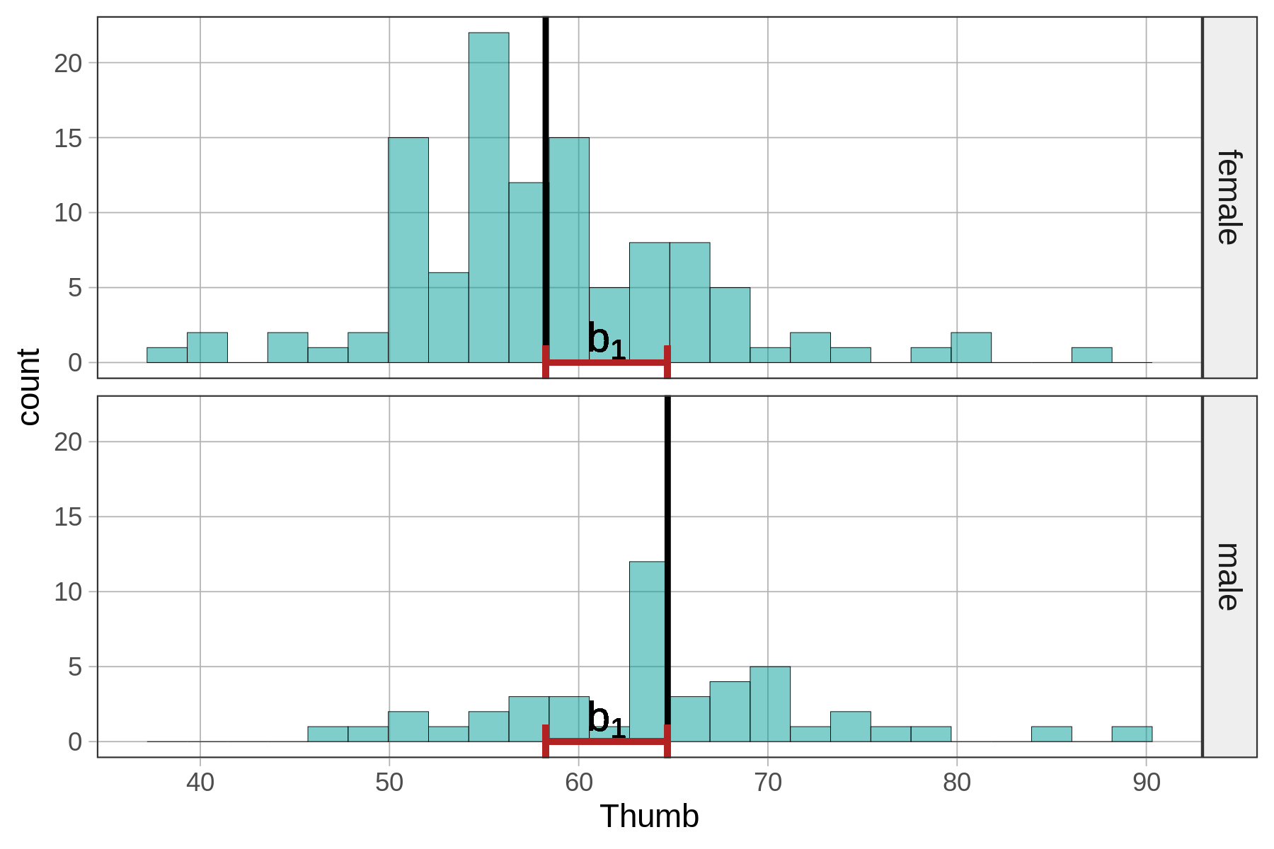
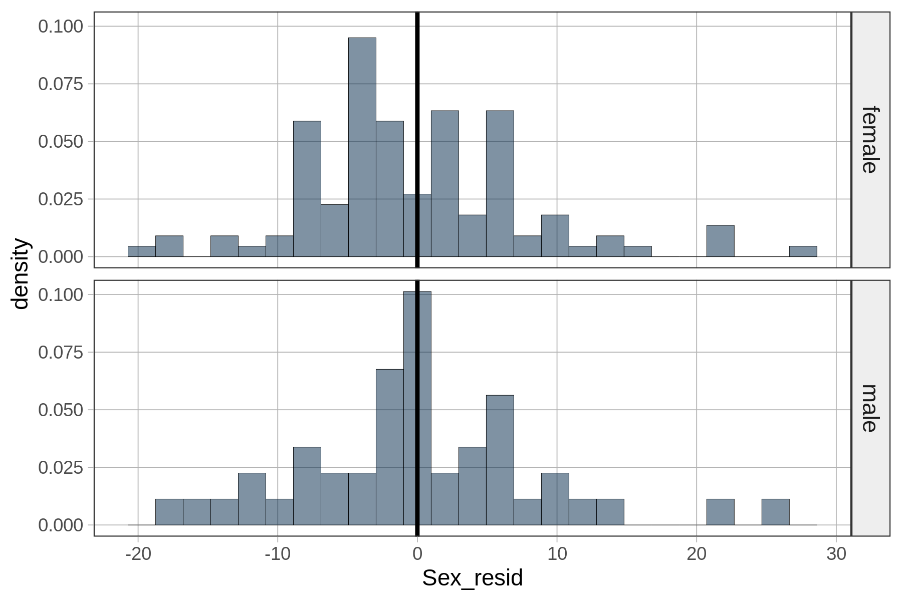
The residuals of the Sex_model represent the variation leftover after taking out the part of the variation that can be explained by Sex. The figures below show the mean Thumb length and mean Sex_resid of the two Sex groups.
mean Thumb of each group
|
mean Sex_resid of each group
|
|---|---|
|
|
|