7.9 Modeling the DGP
We now know how to fit a two-group model to data and to see how much error we can reduce with the two-group model compared to the empty model. But let’s pause for a moment to remember: Our main interest is not in a particular data set, but in the Data Generating Process that generated the data. Even if we have a model that fits our data well, it may not be a good model of the DGP. In fact, it might not even be better than the empty model. Let’s spend some time thinking about this possibility.
Revisiting the Tipping Study
Back in Chapter 4 we learned about an experiment that investigated whether drawing smiley faces on the back of a check would cause restaurant servers to receive higher tips (Rind, B., & Bordia, P. (1996). Effect on restaurant tipping of male and female servers drawing a happy, smiling face on the backs of customers’ checks. Journal of Applied Social Psychology, 26(3), 218-225).
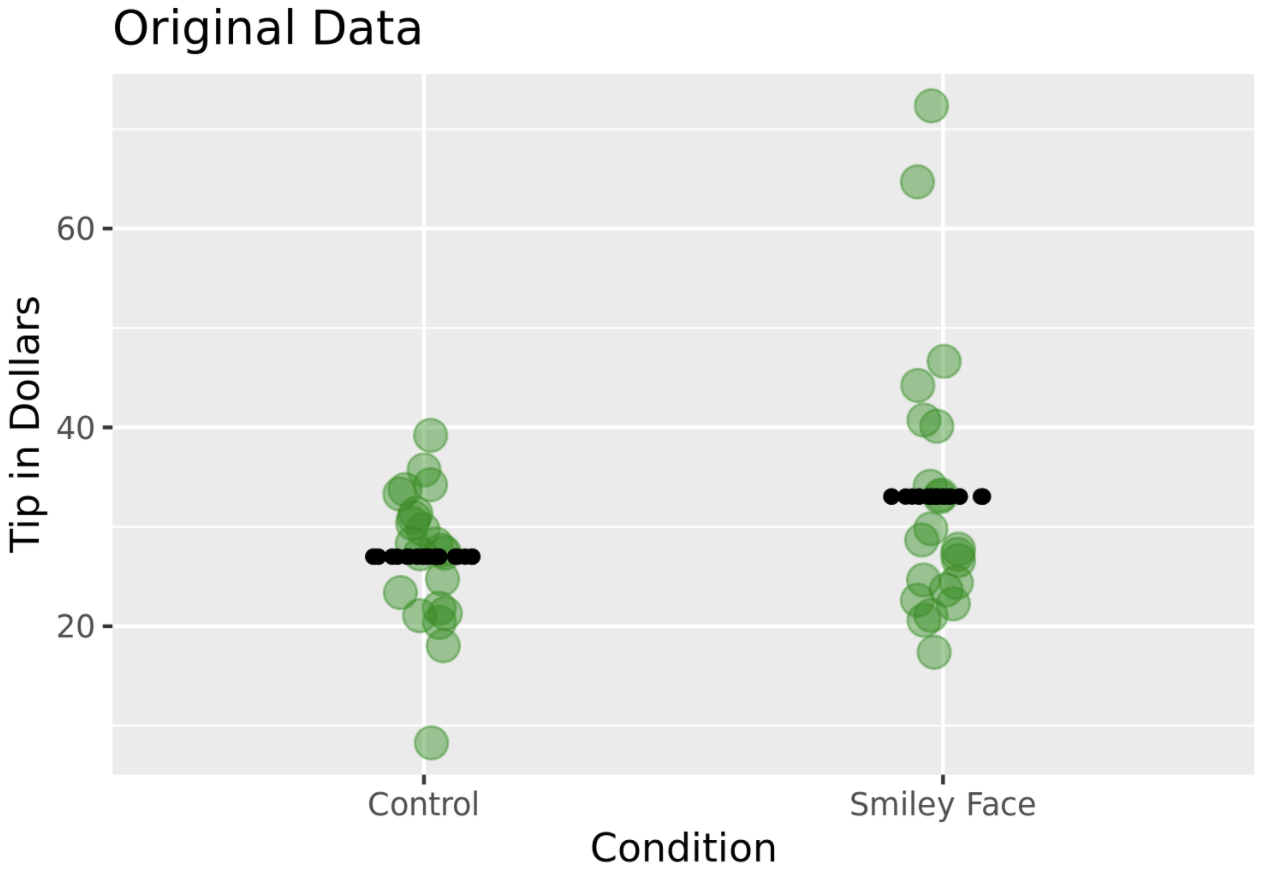
The study was a randomized experiment. A female server in a particular restaurant was asked to either draw a smiley face or not for each table she served following a predetermined random sequence. The outcome variable was the amount of tip left by each table (Tip). Distributions of tip amounts in the two groups (n=22 tables per condition) are shown below.
Use the code window below to fit this two-group model to the data:
\[Y_{i}=b_{0}+b_{1}X_{i}+e_{i}\]
require(coursekata)
# NOTE: The name of the data frame is TipExperiment
lm(Tip ~ Condition, data = TipExperiment)
ex() %>% check_function(., "lm") %>% check_arg("formula") %>% check_equal()In this model, \(b_{1}\) represents our best estimate of the effect of smiley faces on tips, which is +$6. Another way to measure this effect is by calculating PRE, which is included in the ANOVA table below. The PRE of 0.07 means that 0.07 (or 7%) of the total variation in tips is explained by which condition a table is in. (The rest of the variation is explained by other stuff, including randomness.)
supernova(Condition_model)Analysis of Variance Table (Type III SS)
Model: Tip ~ Condition
SS df MS F PRE p
----- --------------- | -------- -- ------- ----- ------ -----
Model (error reduced) | 402.023 1 402.023 3.305 0.0729 .0762
Error (from model) | 5108.955 42 121.642
----- --------------- | -------- -- ------- ----- ------ -----
Total (empty model) | 5510.977 43 128.162Keep in mind, though, that both \(b_1\) and PRE show us the size of the effect in our data. On average, there was a $6 increase in tips caused by drawing smiley faces in our data. But what we really want to know is this: what is the true benefit of drawing a smiley face in the DGP?
$6 is our best estimate of the true benefit, but if we had taken a different sample we would have gotten a different estimate. How much uncertainty is there in our estimate? What might be the true DGP that generated the $6 benefit in our sample?
Although we can calculate the value of \(b_1\), we cannot directly calculate the value of \(\beta_1\). We can estimate it (that’s what \(b_1\) is), but we can’t know it for certain.
We can, however, imagine different possible values of \(\beta_1\), simulate these possible DGPs using R, and use these simulations to help us think about what range of \(\beta_1\)s might be possible given the specific \(b_1\) we calculated. Could the true \(\beta_1\) have been $5? $10? 2.50? Could there be no effect of drawing smiley faces on checks?
If there were no effect of smiley face in the DGP then \(\beta_1\) would be equal to 0. But even if this were the true DGP, we would not expect our sample \(b_1\) to be exactly 0. The reason for this is random sampling variation: if we randomly generate samples from a DGP where \(\beta_1=0\), we will get various estimates of the real effect in the DGP. We would expect these estimates to cluster around 0, but they might vary considerably.
The question is: how much would they vary? Is it possible that a \(b_1\) of $6 could be generated from a DGP where \(\beta_1=0\)? And if is it possible, how likely is it? These are the kinds of questions we can investigate by simulating a DGP where \(\beta_1=0\).
We used the shuffle() function in Chapter 4 to simulate random samples from a DGP with a \(\beta_{1}\) of 0 (i.e., the empty model). We can use shuffle() again, but this time in a more sophisticated way now that we’ve learned how to create a model and calculate \(b_1\).
Hypothetical Thinking
When we use the shuffle() function to simulate the empty model, we are getting our brain to do something it doesn’t naturally do: think hypothetically. We are asking: if the empty model is true, what might the distribution of data look like? What might it look like for one random sample? Or many random samples? If you practice thinking like this, you will find that it can help you draw conclusions about the DGP. But it will take practice, and we will do a lot more of it as we get further through the course.
Let’s look again at the data from the tipping experiment (represented in the jitter plot below). We used black dots to plot the predictions of the two-group model (i.e., the two group means). We also colored one of the tables (Table 1 in the data frame), blue.
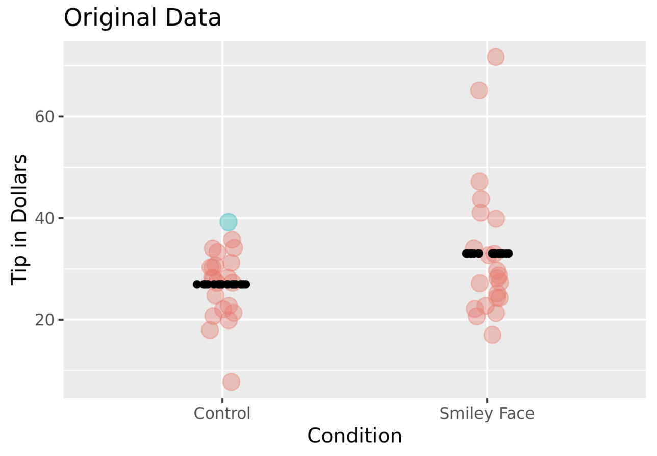
We know that in the actual experiment Table 1 did not get a drawn smiley face and they tipped $39. Let’s think hypothetically for a moment about this: If Table 1 were in the smiley face condition, what would they have tipped? (We know that Table 1 wasn’t in the smiley face condition, but remember, we are thinking hypothetically.) It turns out that the answer to this question depends on which model we believe to be true.
If we believe that smiley face does have an impact on tip amount (TIP = SMILEY FACE + OTHER STUFF), then we would predict, based on our estimate of \(\beta_{1}\), that Table 1 would have tipped an additional $6 if they had been randomly assigned to the smiley face group. But they weren’t, and they didn’t.
What if we believe that smiley face does not have an impact on tipping in the DGP? This would mean that you believe the empty model is true.
If the empty model is true, \(\beta_{1}\) (the effect of smiley face) is equal to 0, so it drops out of the equation. If this model is true, the amount tipped by Table 1 was not affected by which group they were in. Even if Table 1 had been randomly assigned to the smiley face group, they would have tipped the same amount – $39.
Remember: if we assume that the empty model is true (really true in the DGP) then whether or not someone got a smiley face on their check is going to make no difference to how much they tip. Someone who tipped $39 will still tip $39. This is what makes the shuffle() function so powerful, as we will see in the next section.
Simulating the Empty Model (\(\beta_{1}=0\))
The shuffle() command simulates the case where the empty model is true, i.e., \(\beta_1=0\). The basic idea is simple: If there is no effect of smiley face on tips, then any of the tables in the data set could have been in either condition, and they still would have tipped the same amount.
When tables were initially randomly assigned, in the actual experiment, to either get a smiley face or not, the result was only one of the possible random assignments that could have occured. The function shuffle() let’s us do it again (and again), and see what other randomizations would have been possible.
In the figure below, we randomly shuffled all the tables. This time Table 1 happened to be assigned to the smiley face condition. Because we are simulating a random DGP in which smiley faces do not affect tipping, Table 1 still tips the same amount ($39).
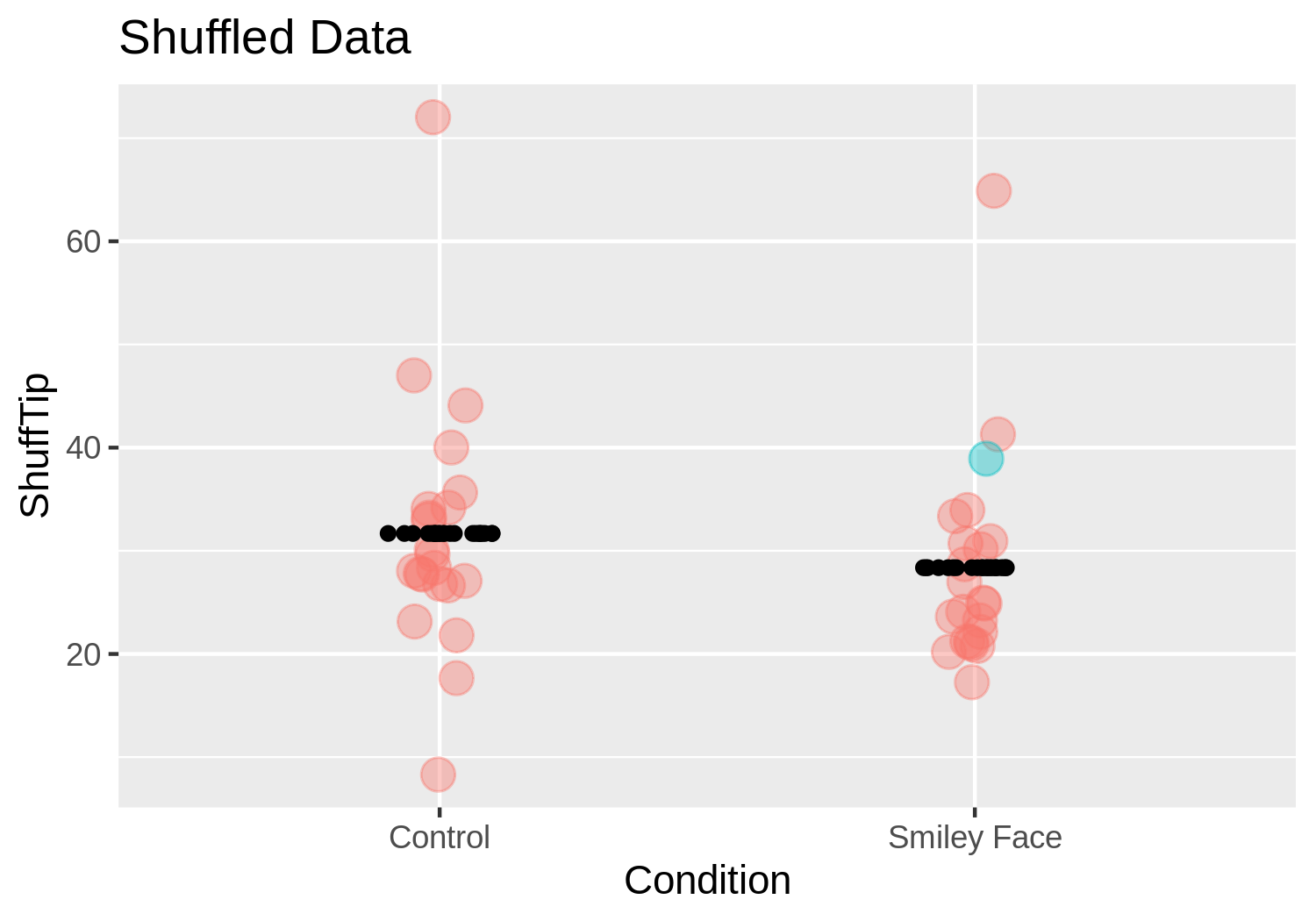
When we shuffle, we are simulating a world in which the only difference between the two groups is due to randomness. Although it’s possible, it won’t usually happen that all the big tipping tables would get randomly shuffled into one group and the smaller tippers into the other group. What’s more likely is that some of the big tipping tables would end up in both groups. For this reason, we would expect the group difference after the shuffle to be close to 0. But because the shuffle is random, it won’t necessarily be exactly 0.
In the plot above, we will still get group differences (the black lines do not have exactly the same value on the y-axis; the two groups don’t have exactly the same means). But the difference is much smaller than in the actual experiment – much closer to 0.
Let’s shuffle the data again, but this time get right to an estimate of what \(b_1\) is for the shuffled data. The code below creates a single shuffled distribution of tips across conditions, fits the two group model, and then, using the b1() function, returns the difference in group means (\(b_1\)).
b1(shuffle(Tip) ~ Condition, data = TipExperiment)Go ahead and add shuffle() to the code in the window below.
require(coursekata)
# shuffle the Tip variable
b1(Tip ~ Condition, data = TipExperiment)
# shuffle the Tip variable
b1(shuffle(Tip) ~ Condition, data = TipExperiment)
ex() %>% check_or(
  check_function(., 'b1') %>%
    check_arg('object') %>%
    check_equal(),
  override_solution_code(., "b1(shuffle(Tip) ~ shuffle(Condition), data = TipExperiment)") %>%
    check_function(., 'b1') %>%
    check_arg('object') %>%
    check_equal(),
  override_solution_code(., "b1(Tip ~ shuffle(Condition), data = TipExperiment)") %>%
    check_function(., 'b1') %>%
    check_arg('object') %>%
    check_equal()
)Adding the do() function in front of the code above lets us repeat this random process multiple times, generating a new \(b_1\) each time.
Try modifying the code in the window below to produce 10 shuffles of the tips across conditions, and 10 estimates of \(\beta_1\).
require(coursekata)
# modify to produce 10 shuffled b1s
do( ) * b1(shuffle(Tip) ~ Condition, data = TipExperiment)
# modify to produce 10 shuffled b1s
do(10) * b1(shuffle(Tip) ~ Condition, data = TipExperiment)
ex() %>%
  check_function('do') %>%
  check_arg('object') %>%
check_equal() b1
1 -3.7727273
2 -2.6818182
3 -1.4090909
4 -2.6818182
5 -4.6818182
6 2.0454545
7 -0.1363636
8 -1.1363636
9 0.5909091
10 4.6818182The ten \(b_1\) estimates that resulted when you ran the code will not be exactly the same as the estimates we got (shown above). This is because each random shuffle of the data will differ. But notice that some of these shuffled \(b_1\)s are positive and some are negative, some differences are quite different from 0 (e.g., 4.68 and -3.77) and some are fairly close to 0 (e.g., -0.13). Feel free to run the code a few times to get a sense of how these \(b_1\)s can vary.
If we continue to generate random \(b_1\)s, we would start to see that although they are rarely exactly 0, they are clustered around 0. Why is this? It’s because shuffle simulates a DGP in which there is no effect of smiley face on tips, and in which the tables would have tipped the same amount even if they were put into the other condition.
Bear in mind: Each of these \(b_1\)s results from a random process that has nothing to do with whether the table actually got smiley faces or not. The shuffle() function mimics a DGP where \(\beta_1=0\). Sometimes the DGP is called “the parent population” because when it generates \(b_1\)s, these “children” tend to resemble their parent.
Using Simulated \(b_{1}\)s to Understand Our Sample Better
Now let’s see how we can use the \(b_1\)s we simulated assuming the empty model of the DGP to help us interpret the \(b_1\) that was estimated from data in the actual experiment.
By simulating the range of \(b_1\)s that can be generated by the empty model, we can then ask: how likely is it that the sample \(b_1\) observed in the experiment could have been generated by the empty model? Does it look like it fits in that distribution of \(b_1\)s, or does it look like it doesn’t? If it doesn’t fit, we might conclude that the empty model is not true, and that the smiley face model is better.
To see how this works, let’s look again at the 10 \(b_1\)s we simulated above from the empty model. This time, let’s sort them in order, from smallest to largest.
           b1
1  -3.7727273
2  -3.2272727
3  -1.6818182
4  -1.6818182
5  -1.5000000
6  -0.5000000
7   0.1363636
8   2.7727273
9   3.6818182
10  6.9545455
One of the 10 simulated \(b_1\)s is larger than 6, while the other 9 are smaller. What does this mean? It seems to indicate that while it is possible that the observed \(b_1\) in the experiment could have been generated from a DGP in which the true \(\beta_1=0\), it is not common to see a \(b_1\) higher than 6.
Based on this, would we want to rule out the empty model as being the true model of the DGP? That’s a hard call, and one we will return to in Chapter 9. For now, just note that seeing the observed \(b_1\) in the context of other \(b_1\)s that could have been generated from the empty model, helps us to think more critically about how we should interpret the results of the tipping study.
Connecting \(\beta_1\) to \(P\!R\!E\)
We have seen that when we use shuffle to randomly generate \(b_1\)s from the empty model, the resulting \(b_1\)s will tend to cluster around 0. This makes sense, because there is, in fact, no effect of smiley face on tips if the empty model is true.
This same logic can be applied to other measures of effect size, for example, PRE. If we want, we can shuffle the data again, but instead of calculating \(b_1\) for the shuffled data we can calculate PRE.
We can apply the same logic we used above for interpreting \(b_1\) to the interpretation of PRE, which was roughly .07 in the smiley face study. To get the output below, we shuffled the data 10 times (assuming the empty model is true), calculated the PRE for each shuffle, and then arranged the PREs in order from low to high. We used this code:
bunch_of_PREs <- do(10) * PRE(shuffle(Tip) ~ Condition, data = TipExperiment)
arrange(bunch_of_PREs, PRE)
PRE
1 0.005645757
2 0.005645757
3 0.008351101
4 0.014355646
5 0.015345406
6 0.016368158
7 0.016368158
8 0.040419328
9 0.047215681
10 0.078949444Similar to when we simulated \(b_1\)s, only one of the simulated PREs from the empty model was as large as the one observed in the experiment, which was .07. What does this mean? It means that getting an effect as large as a PRE of .07 is not very common when PREs are generated from the empty model.
Does this mean we can reject the empty model? Maybe. We will address this question in much more detail in Chapter 9. For now, just keep in mind that in order to think about what our data say about what’s really true about the DGP, we will need to consider (and eventually quantify) sampling variation.