7.1 Specifying the Model

Reviewing the Empty Model

In the previous chapters we introduced the idea of a statistical model as a function that generates a predicted score for each observation. We developed what we called the empty model, in which we use the mean as the predicted score for each observation.

We represented this model in GLM notation like this:

$$Y_i=b_0+e_i$$

where $b_0$ represents the mean of the sample on the outcome variable.

It is important to remember that $b_0$ is just an estimate of the true mean in the population or Data Generating Process. To distinguish the true mean, which is unknown, from the estimate of the true mean we construct from our data, we use the Greek letter ${\beta }_0$ and write the empty model of the DGP like this:

$$Y_i={\beta }_0+{ϵ}_i$$

The empty model is called a one parameter model because we only need to estimate one parameter (${\beta }_0$) in order to generate a predicted score for each observation.

Because we don’t know for sure what the true mean (${\beta }_0$) is, we also can’t know for sure how far a particular data point deviates from the true mean. For this reason, we also use a Greek letter (${ϵ}_i$) to refer to each observation’s error from the true mean.

In the case of thumb length, this model states that the DATA (each data point, represented as $Y_i$, which is each person’s measured thumb length), can be thought of as having two components: MODEL, represented as $b_0$, which is the mean thumb length for everyone (usually called the Grand Mean); plus ERROR, which is each person’s residual from the model, represented by $e_i$.

(Note: We use the term Grand Mean to refer to the mean of everyone in the sample in order to distinguish it clearly from other means, such as the mean for males or the mean for females.)

When we use the notation of the General Linear Model, we must define the meaning of each symbol in context. $Y_i$, for example, could mean lots of different things, depending on what our outcome variable is. But we will always use it to represent the outcome variable. Because we are talking about the outcome of Thumb length here, we can also write the empty model like this:

$${Thumb}_i=b_0+e_i$$

NOTE: In this chapter and the next, we will generally use the non-Greek notation because our focus will be on estimating models from data. Later in the book we will return to the world of the DGP and ask how we can use the models we estimate to help us make inferences about the Data Generating Process.

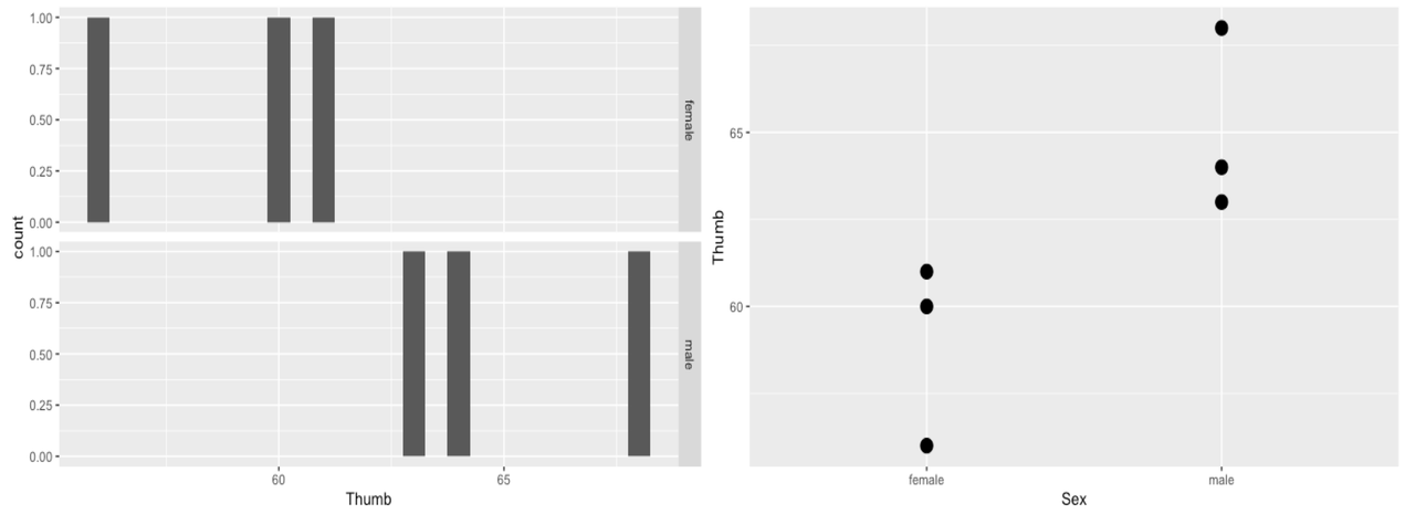
It’s useful to illustrate the null model (or empty model) with our TinyFingers data set. TinyFingers, you will recall, contains six people’s thumb lengths, three males and three females, randomly selected from our complete Fingers data set.

TinyFingers

     Sex Thumb
1 female    56
2 female    60
3 female    61
4   male    63
5   male    64
6   male    68

We could represent the distribution of the six thumb lengths, broken down by Sex, using a faceted histogram (left panel, below). Or, we could use a scatterplot (gf_point(), as shown in the right panel), which might be clearer with such a small data set.

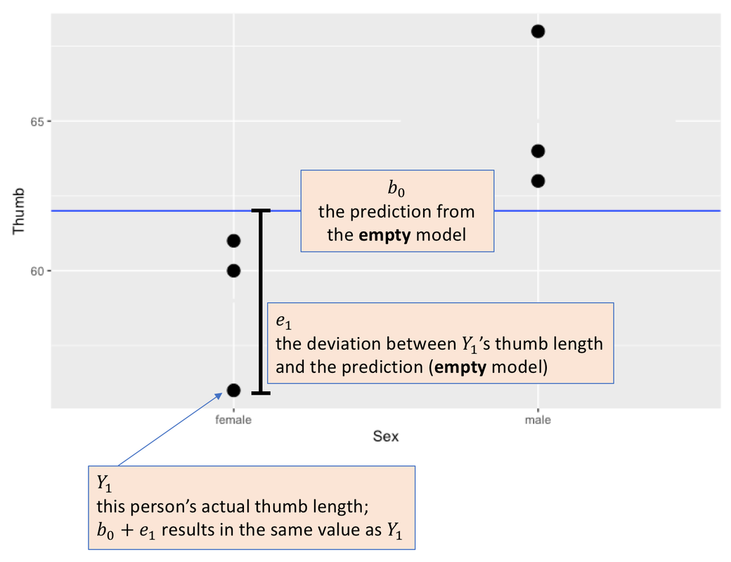
In the scatterplot below, the Grand Mean of the distribution, ignoring sex, is represented by the blue line. The Grand Mean is the model prediction for all observations under the empty model. Whether someone is male or female, their predicted thumb length ($b_0$) is 62 millimeters. Each person’s actual measured thumb length ($Y_i$) would be equal to 62 ($b_0$) plus their error or residual from the model prediction ($e_i$).

Adding an Explanatory Variable to the Model

Now let’s add an explanatory variable, Sex, into the model. In the Sex model, which includes sex as an explanatory variable, we model the variation in thumb length with two numbers: the mean for males (65), and the mean for females (59). The model still generates a predicted thumb length for each person, but now the model generates a different prediction for a male than it does for a female.

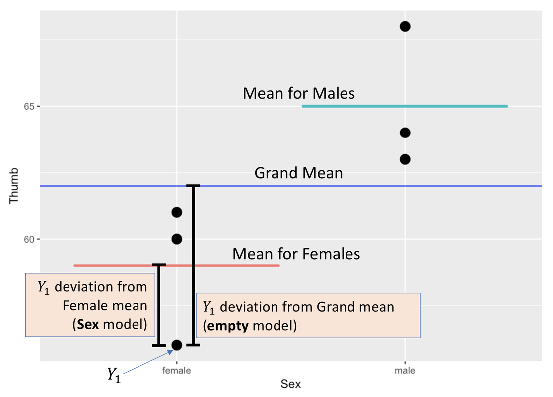
Error is still measured the same way, as the deviation of each person’s measured thumb length from their predicted thumb length. But this time, the error is calculated from each person’s group mean (male or female) instead of from the Grand Mean (see figure above).

Whereas the empty model was a one-parameter model (we only had to estimate one parameter, the Grand Mean), the Sex model is a two-parameter model. One of the parameters is the mean for males, the other is the mean for females.

There are actually a few ways you could write this model; we will write the model of the DGP like this:

$$Y_i={\beta }_0+{\beta }_1{X}_i+{ϵ}_i$$

Replacing the parameters with their estimates, we write the model we are estimating with our data like this:

$$Y_i=b_0+b_1{X}_i+e_i$$

We can also write it like this:

$${Thumb}_i=b_0+b_1{Sex}_i+e_i$$

In this equation, $Y_i$ is still the thumb length for person i (DATA), and $e_i$ is still the error for person i (ERROR), i.e., the deviation of the thumb length of person i from the thumb length predicted by the model. The part of the equation in between DATA and ERROR ($b_0+b_1{X}_i$) is the MODEL part of DATA = MODEL + ERROR, and it requires a bit of unpacking.

Interpreting the GLM Notation for a Two-Group Model

In the two-group model, the model statement, $b_0+b_1{X}_i$, still represents each person’s predicted thumb length. But in this case, the model makes a different prediction for each person depending on their sex, $X_i$. This prediction ($b_0+b_1{X}_i$) plus error ($e_i$) will equal each person’s actual thumb length ($Y_i$).

Let’s unpack the GLM notation to see how it generates the two possible model predictions. In the two-group model, $b_0$ no longer represents the Grand Mean (62), but instead represents the mean for one of the groups. For example, $b_0$ might represent the mean thumb length for females, which, in the TinyFingers data frame, is 59.

If $b_0$ represents the mean for females, then $b_1$ represents what you would add on to the mean for females in order to get the mean (i.e., the model prediction) for males. As such, $b_1$ would represent the difference, or increment, in means between females and males. In the TinyFingers data, that increment is 6 mm, meaning that if you add 6 mm to the mean for females you will get the mean for males.

Here is how we would rewrite the model to include the estimated parameters:

$$Y_i=59+6X_i+e_i$$

You can also write Thumb and Sex instead of writing Y and X:

$${Thumb}_i=59+6{Sex}_i+e_i$$

Now let’s see how these two parameter estimates (59 and 6) work inside the overall model ($Y_i=b_0+b_1{X}_i+e_i$).

$X_i$ is going to represent our explanatory variable, which is Sex. The subscript i reminds us that each person will have their own value on this variable (i.e., each person is either female or male). In order to make the model add up, we code $X_i$ as 0 for females and 1 for males. (This method of coding the explanatory variable is called “dummy coding”. There are other methods, but this is the one we use in this book.)

Let’s see what would happen if we used this model to predict a female’s thumb length. If someone is female, she would be coded 0 for $X_i$. $b_1\ast X_i$ would then be 6 times 0, which means the model would assign her a predicted thumb length of $b_0$ (which is 59), plus 0. This adds up to 59, the mean for females.

Let’s consider what would happen if we asked this model to predict a male’s thumb length. If someone is male, he would be coded 1 for $X_i$. A male’s thumb length would be 59 + (6 * 1), which means the model would assign him a predicted thumb length of 65, the mean for males.

Under this model, as expected, males would all end up with one predicted thumb length (65, the mean for males, or $b_0+b_1\ast 1$), and females would all end up with a different predicted thumb length (59, the mean for females, or $b_0+b_1\ast 0$).

Comparing the Two-Group Model With the Empty Model

We’ve discussed what happens when $X_i$ equals 0 or 1, but what if ${\beta }_1=0$? This is worth thinking about, because it’s exactly what differentiates the two-group model from the empty model. Let’s compare the two:

Two-group model: $Y_i={\beta }_0+{\beta }_1{X}_i+{ϵ}_i$

Empty model: $Y_i={\beta }_0+{ϵ}_i$

In the two-group model, if ${\beta }_1=0$, it means that there is no mean difference between the two groups in the DGP. If this is the case, then ${\beta }_1{X}_i$ drops out of the equation, because if ${\beta }_1=0$, then ${\beta }_1\ast X_i$ would be equal to 0, no matter what value the variable $X$ takes on (0 or 1).

Notice, then, that if ${\beta }_1{X}_i$ drops out of the equation, we are left with just the empty model: $Y_i={\beta }_0+{ϵ}_i$

A Final Note on Error

Note that we are broadening our definition of error from the way we thought of it for the empty model. For the empty model, error was the residual from the mean (i.e., the Grand Mean). Now we need to expand our thinking a bit, seeing error as the residual from the predicted score, which may not necessarily be the Grand Mean.

Of course, under both models (empty and two-group) the error is the residual from the predicted score under the model. It so happens that in the empty model, that predicted score is the Grand Mean. In the two-group model, the error is the residual from the male mean if you are male, or the female mean if you are female.

No matter how complex our models become, error is always defined as the residual, for each data point, from its predicted score under the model.