9.10 Using Shuffle to Interpret the Slope of a Regression Line

Simulating $b_1$ Under the Empty Model (Revisited)

In Chapter 7, we spent some time revisiting the tipping study. We modeled the data using a two-group model, and found tables that got a smiley face on the check tipped $6 more, on average, than those that didn’t.

Although there was a $6 advantage of smiley face in our data, what we really want to know is: what is the advantage, if any, in the Data Generating Process? Could the $6 advantage we observed have been generated randomly by a DGP in which there is no advantage (i.e., a model in which ${\beta }_1=0$?

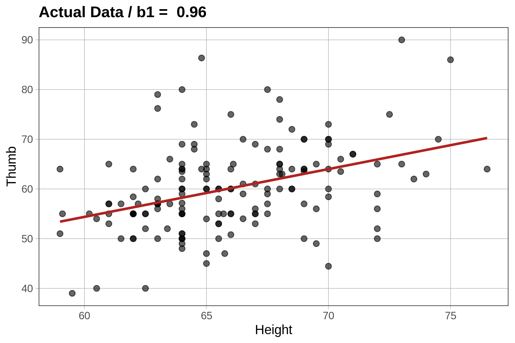
It turns out we can ask the same question with a regression model, in which ${\beta }_1$ is a slope instead of a group difference. When we fit a regression model, regressing Height on Thumb, our best fitting estimate of the true slope (${\beta }_1$) was 0.96. But could this relationship in our data have been generated by a DGP in which ${\beta }_1=0$?

We can ask this question by using the shuffle() function to simulate a DGP in which the empty model is true. This time, instead of shuffling which condition tables are in we will shuffle one of the two variables in our model, Thumb or Height. In this case, it doesn’t really matter which one we shuffle; we could even shuffle both. In general, it’s best to shuffle the outcome variable.

By randomly shuffling one of these variables we are simulating a DGP in which there is absolutely no relationship between the two variables, and in which any apparent relationship that appears could only be due to randomness, and not a real relationship in the DGP. If the relationship in our data was a real one, shuffling breaks it, and it isn’t real any more!

Let’s see how this works graphically. The code produces a scatterplot of Thumb by Height along with the best fitting regression line. We added in a line of code (gf_labs()) that prints the slope estimate as a title at the top of the graph.

sample_b1 <- b1(Thumb ~ Height, data = Fingers)

gf_point(Thumb ~ Height, data = Fingers) %>%
 gf_lm(color = "firebrick")%>%
 gf_labs(title=paste("Actual Data / b1 = ", round(b1(Thumb ~ Height, data=Fingers),digits=2)))

Now let’s see what happens if we shuffle the variable Height before we produce the graph and best-fitting line. We accomplish this by simply adding a line of code right before the gf_point() that creates a new variable named ShuffThumb, and then plotting ShuffThumb by Height.

Fingers$ShuffThumb <- shuffle(Fingers$Thumb)
shuffled_b1 <- b1(ShuffThumb ~ Height, data = Fingers)
 
gf_point(ShuffThumb ~ Height, data = Fingers) %>%
   gf_lm(color = "purple") %>%
   gf_labs(title=paste("Shuffled Data / b1 = ", round(shuffled_b1,digits=2)))

We’ve added the shuffle code into the window below, and also changed the gf_labs() code to title the graph Shuffled Data instead of Actual Data. Go ahead and run the code and see if it does what you thought it would. Run it a few times, and see how it changes.

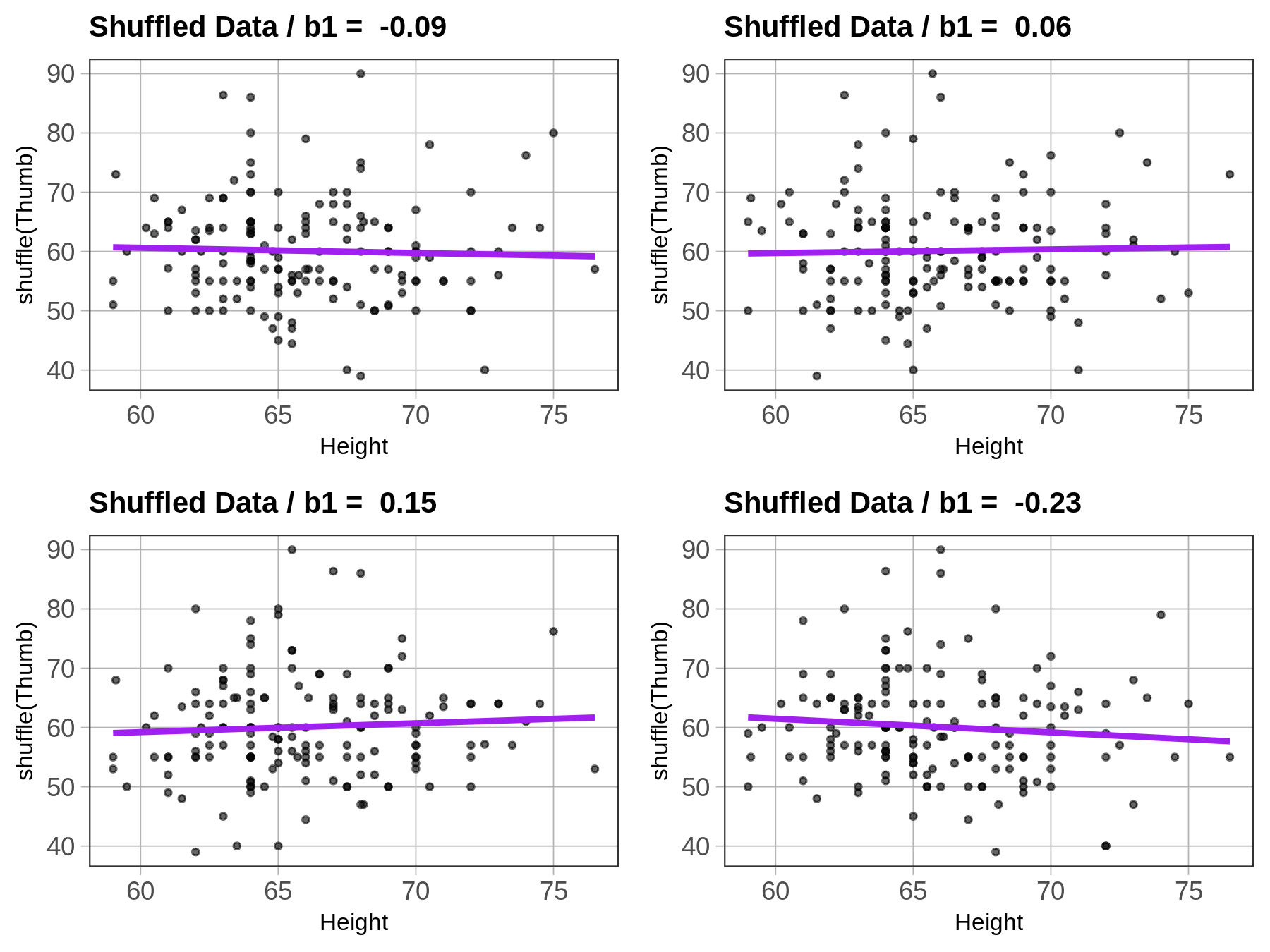
You can see that the $b_1$s vary each time you run the code, but they seem to be clustered around 0, a little negative or a little positive. This makes sense because we know that the true ${\beta }_1$ in this case is 0. And how do we know that? Because we know that any relationship between Thumb and Height is purely random due to the fact that we shuffled one of the variables randomly.

Instead of producing a graph, we can also just produce a $b_1$ directly by using the b1() function together with shuffle():

b1(shuffle(Thumb) ~ Height, data = Fingers)

Use the code window below to do this 10 times and produce a list of 10 $b_1$s.

Here are the 10 $b_1$s we generated (your list would differ, of course, because each one is based on a new random shuffle):

             b1
1   0.059185509
2  -0.013442382
3   0.027153003
4  -0.008801673
5   0.007565065
6   0.219193990
7  -0.132471001
8   0.035662413
9  -0.157540915
10 -0.035323177

As we did previously for the tipping study, we can use this list of $b_1$s generated by random shuffles of the data to help us put our observed $b_1$ of 0.96 in context. Here we arranged these $b_1$s in order (smallest to largest) to make it easier to compare them to our sample $b_1$.

             b1
1  -0.157540915
2  -0.132471001
3  -0.035323177
4  -0.013442382
5  -0.008801673
6   0.007565065
7   0.027153003
8   0.035662413
9   0.059185509
10  0.219193990

As you can see, these randomly generated $b_1$s cluster around 0 – roughly half are negative and half are positive. This makes sense given that their parent (${\beta }_1$) was equal to 0. None of them come anywhere close to being as high as our sample estimate of 0.96.